Counting and cardinality

Recall that information is often in the form of identifying a state/outcome among a set of states/possibilities. In this context, the size of the set of the states is an important property. We devote this section to learn more about the sizes of sets.

Finite and infinite sets

First, let us define two types of sets. Sets containing a finite number of elements are called finite sets. For such sets, there is a natural number that gives the number of elements. For example, the set of prime numbers less than 10, {2,3,5,7}, has 4 elements.

An infinite set is one that has an infinite number of elements. In other words, there is no natural number that can describe the size of an infinite set; we can always present more elements than the proposed number.

Some examples of infinite sets:

• Natural numbers: \(\mathbb N = \{0,1,2,\dotsc\}\).
• Integers: \(\{0,1,-1,2,-2,\dotsc\}\)
• Real numbers, or equivalently points on the real line
• The set of points in the interval from 0 to 1

Size and Cardinality

There are different ways that we can define the notion of size for sets. The most relevant to us is cardinality of a set. For a finite set, the cardinality is simply the number of elements in the set.

What about infinite sets? Do all infinite sets have the same number of elements, for example natural and real numbers? Cardinality is also generalized to infinite sets, helping us classify infinite sets in a way that has implications for storing information, as we’ll discuss below. We use the terms size and cardinality interchangeably, even though one the former is an informal concept while the latter is mathematical term.

Counting the elements of finite sets

Basic Counting Rules

When the elements of a finite set are not given explicitly, we may need to compute the size of the set. The following two rules can be helpful for this task.

Other Counting Techniques

We will now see some more advanced techniques. These are essentially shorthands for a specific way of applying the rules of sum and product to specific situations.

Drawing with Replacement

We call this drawing with replacement.

For $N$ things, drawing $K$ items with replacement gives: \(N^K\) possibilities. Note that here the order of the items matter. For example, $(A\heartsuit, K\spadesuit)$ is different from $(K\spadesuit, A\heartsuit)$.

Darwing without replacement

Usually, when we draw from a deck of cards, we don’t replace the card. Assume order still matters.

A bit of notation before we proceed. We show the product $1\times2\times\dotsm\times n$ as $n!$ (read $n$ fatorial). In other words,

We call this an ordered draw without replacement.

For $N$ things, choosing $K$ items in order gives:

possibilities. Using the factorial notaiton, we can write this more compactly as

possibilities.

Permutations

An arrangement of $N$ items is called a permutation. There are

ways to arrange $N$ items. (This is a special case of ordered drawing without replacement, where we draw all $N$ items.)

There are

ways to arrange a full deck of cards!

Aside: How Large is $52!$?

If everyone who has ever lived shuffled a deck once every second since the beginning of time, the number of permutations we could go through is approximately:

So not even close to the number of possible premutations. This means if you randomly shuffle a deck of card, you have an object in your hand that almost surely has never existed in that configuration before!

Combinations

Up to this point, we have assumed that order does matter. But this is not always the case. The most common situation is when we want to choose $K$ items out of a set of $N$ items, like choosing which 5 friends to invite to your birthday from a set of 10 friends, with order not being important. Another example is that in a game of card, the hand ${A\heartsuit, K\spadesuit}$ is the same as ${K\spadesuit, A\heartsuit}$. We call this an unordered draw without replacement, or a combination.

The number of possible ways that we can choose $K$ items from a set of $N$ itmes is mathematially shown as \(\binom{N}{K}\) (read $N$ choose $K$). We have

This formula can be understood intuitively as follows: if we first consider the scenario where order matters, there are

ways to choose $K$ items from $N$. However, each group of $K$ items can be arranged in $K!$ different ways. Since order doesn’t matter in combinations, we have overcounted each group by a factor of $K!$. Dividing by $K!$ corrects for this overcounting, leading to the formula: \(\binom{N}{K} = \frac{N!}{K!(N-K)!}.\)

More (Advanced) Exercises

Counting Principles Summary

Infinite sets: countably infinite vs uncountable

Some sets are infinite, or equivalently have an infinite number of elements. Infinity is not a number, but it is convenient to treat it as a number sometimes. However, not all infinities are created equal. Some infinite sets are much bigger than the other ones. One possible way to classify infinite sets is to divide them into countably infinite sets and uncountable sets. Uncountable sets are unimaginably bigger than countably infinite sets.

To understand what the difference is, we need to learn about bijections. A bijection between two sets \(A\) and \(B\) is a function that maps each element of \(A\) to exactly one element of \(B\) and for each element of \(B\), there is an element of \(A\) that is mapped to it.

So roughly speaking a bijection means the same size. This is very natural for finite sets but also holds for infinite sets. For example, there is a bijection between the set of even numbers \(\mathbb E=\{0,2,4,6,8,\dotsc\}\) and the set of natural numbers \(\mathbb N\), as shown by the \(f(x)=2x\).

So even numbers and natural numbers have the same cardinality. Informally, there are the same number of even numbers as there are natural numbers 🤯.

In other words, we can “count” the elements of a countably infinite set, labeling them 0, 1, 2, and so on (you can also start counting from 1). Yet another way to show a set is countably infinite is to “list” all its elements, in a way that every element appears is the list. For even numbers, the list can be:

[0,2,4,\dotsc]

A countable set is either finite or countably infinite. Typically though, when people say countable, they mean countably infinite.

Rationals and reals

So far we have only seen countable sets. Rationals and reals seem like good candidates for being uncountable. Between any two rational numbers there exists another rational number so this suggests that it might be difficult to list all rational numbers. It turns out, however, that the rational numbers are countable.

So the set of rational numbers and the set of natural numbers have the same size 🤯🤯

But real numbers are uncountable. It can be proven that any strategy for listing all real numbers will fail. One way to prove this is Cantor’s diagonal argument.

Beyond naive set theory

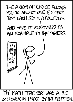
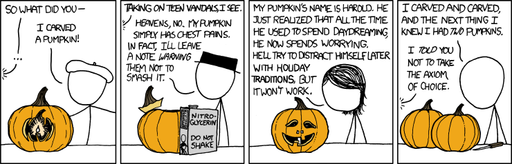
Set theory is a fascinating topic, with many surprising (and controversial) results, especially when dealing with uncountable sets. Click on images below to learn about the axiom of choice, and how not to carve pumpkins.

Image credit: XKCD

Cardinality and information

Recall that information is determining one state/possibility among a set of states/possibilities. The cardinality of the set has implications on whether we can represent the corresponding information on a computer.

• If the set of possibilities is countable, information can be represented on a computer (or a piece of paper). That is, given sufficient memory, we can store the information.
• If the set is uncountable, like real numbers, there are going to be some possibilities for which we do not have a representation and cannot be stored on any computer.