Multivariate Random Variables

Part 3: How can we make accurate predictions based on data, and how accurate can they be?

Probabilistic Machine Learning

University of Virginia
Farzad Farnoud

Chapter 4

This chapter is about several random quantities studied together: how they vary jointly, and how observing some of them helps predict the others. It belongs to the part of the course that asks how we can make accurate predictions from data, and how accurate those predictions can be.

A parent marking a child's height on a door frame

AI-generated illustration

From data to prediction

Question: How can we predict a child's adult height?

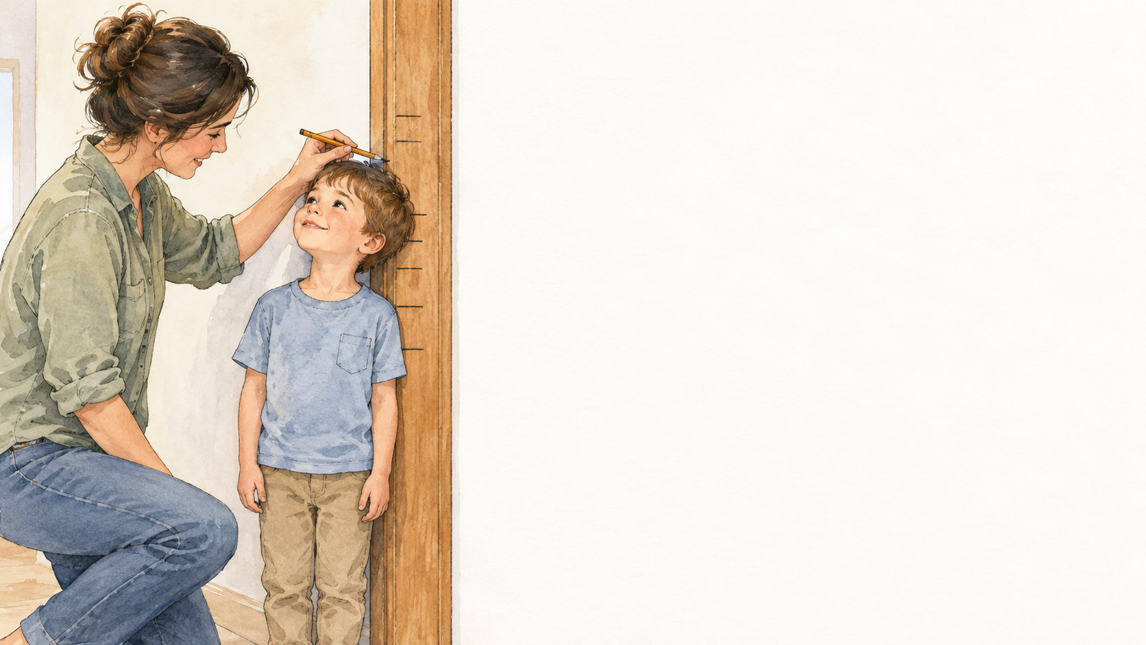
Can we use the parents' heights?

What we need:

12A model of the relationship between the known (the parents' heights) and the unknown (the child's height). Today's model: the multivariate Gaussian.
3A method for predicting the unknown from the known in that model.
4A way to find the model from data.

Running example: $X_1$ a parent's height and $X_2$ the adult child's height, in standard deviations from their means, jointly Gaussian with correlation $\rho=0.5$ (illustrative, not measured data).

Take predictions without giving the formula. Return to this observation during conditioning. Say we want to predict a child's adult height. It is strongly related to the parents' heights, so we would like to use them. To do that, we need three things. First, a model of how the heights vary together. Ours is the multivariate Gaussian, which the central limit theorem makes natural for a quantity built from many small effects. Second, a way to predict the unknown height from the known ones within that model. Third, a way to estimate the model from data. Throughout, X one is a parent's height and X two the child's adult height, both in standard deviations from their means, with correlation one half; these numbers are illustrative. Before going on, make a guess: if a parent is unusually tall, how tall do you expect the child to be?

The mind map of the deck. Entering pulls back from the opening slides to the whole map; the click zooms into part 1. This map is the outline of the chapter. Part one builds the tools for any random vector: the mean, the covariance matrix, and how linear transformations change them. Part two introduces our model, the Gaussian random vector. Part three uses conditioning to turn the model into predictions, and part four estimates the model from data. We start with part one, which applies to any random vector, Gaussian or not.

Mean of a random vector

\[\bX=\begin{pmatrix}X_1\\X_2\end{pmatrix},\qquad \bmu=\E\bX=\begin{pmatrix}\E X_1\\\E X_2\end{pmatrix}\] Each dot is one pair. An observed pair is a deterministic vector $\bx$.

Here $\bmu=(1,1)^T$. The arrow $\bx-\bmu$ is the pair's deviation from the center.

Question: Add a fixed vector $\bb=(-3,1)^T$ to every pair. What happens to the mean, and to the deviation $\bx-\bmu$?

Every point and the mean move by the same amount: $\E[\bX+\bb]=\bmu+\bb=(-2,2)^T$. The deviations $\bx-\bmu$ stay the same.

Ask which part of the picture describes variability: the arrow from the mean to a point. A random vector stacks several random variables, here a parent's height and a child's height. We work in two dimensions because they are easy to draw; everything carries over to many dimensions. The mean of a random vector is the vector of the individual means. Each dot on the right is one pair drawn from the distribution, and an observed pair is an ordinary vector, written lowercase x. Here the mean is at one, one. The teal arrow from the mean to one point is that point's deviation, x minus mu. The covariance will be built from these deviations. Now shift every pair by the same vector b, three units to the left and one up. What happens to the mean, and to the deviation arrow? Predict before the next step. Everything moves together. The mean lands at minus two, two, and the arrow from the mean to the point keeps its length and direction. A shift changes the center and leaves the spread around it untouched, and the spread is what the covariance measures.

Covariance matrix of a two-dimensional vector

For $\bX=(X_1,X_2)^T$ with mean $\bmu=(\mu_1,\mu_2)^T$:

\[\mK=\E[(\bX-\bmu)(\bX-\bmu)^T]\]

\[(\bX-\bmu)(\bX-\bmu)^T=\begin{pmatrix}\textcolor{#A0521B}{(X_1-\mu_1)^2}&\textcolor{#6A3D9A}{(X_1-\mu_1)(X_2-\mu_2)}\\\textcolor{#6A3D9A}{(X_2-\mu_2)(X_1-\mu_1)}&\textcolor{#A0521B}{(X_2-\mu_2)^2}\end{pmatrix}\]

Take the expectation entry by entry:

\[\mK=\begin{pmatrix}\textcolor{#A0521B}{\var(X_1)}&\textcolor{#6A3D9A}{\cov(X_1,X_2)}\\\textcolor{#6A3D9A}{\cov(X_2,X_1)}&\textcolor{#A0521B}{\var(X_2)}\end{pmatrix}\]

The two off-diagonal entries are equal, so $\mK$ is symmetric. In $d$ dimensions, $\mK_{ij}=\cov(X_i,X_j)$ and $\mK_{ii}=\var(X_i)$. In one dimension, the variance averages the squared deviation from the mean. For a random vector, the deviation X minus mu is itself a vector, and squaring becomes multiplying it by its own transpose: a column times a row, which gives a matrix. The covariance matrix K is the average of that matrix. In two dimensions, this matrix holds each coordinate's squared deviation on the diagonal and the product of the two deviations off the diagonal. Averaging entry by entry turns the diagonal into the two variances and the off-diagonal entries into the covariance of X one and X two. The diagonal says how much each coordinate varies on its own; the off-diagonal says how the two vary together. The two off-diagonal entries are equal, so K is symmetric. In any dimension, the entry in row i and column j is the covariance of X i and X j, and the diagonal holds the variances.

Sign of the covariance

\[\cov(X_1,X_2)=\E[(X_1-\mu_1)(X_2-\mu_2)]\]

The off-diagonal entry averages the product of the two deviations; with $\bmu=\bzero$ that product is $x_1x_2$.

Question: Which quadrants hold more of the points, and what sign will the average product $x_1x_2$ have?

The positive products outweigh the negative ones in this model.

\[\mK=\begin{pmatrix}1&0.5\\0.5&1\end{pmatrix},\qquad \rho=\frac{\cov(X_1,X_2)}{\sigma_1\sigma_2}=0.5\] It is positive when the two deviations tend to have the same sign and negative when they tend to have opposite signs.

Covariance requires finite second moments. The notes call E[XY^T] a correlation matrix: it is an uncentered second moment, distinct from the normalized correlation coefficient rho here. Cov(X,Y)=E[XY^T]-E[X]E[Y]^T. The 400 dots are a sample; their average product is close to, not equal to, 0.5. The sign of the covariance tells us whether two coordinates tend to move together or in opposite directions. The covariance is the average product of the two deviations, and here, with the mean at zero, each point contributes x one times x two. The cloud on the left is a sample from our running model. The product is positive in the upper-right and lower-left quadrants, where the two coordinates have the same sign, and negative in the other two. Which quadrants hold more of the points, and what sign will the average have? Predict before the next step. Coloring each point by the sign of its product settles it: two hundred ninety-two products are positive and one hundred eight negative, with an average of about one half. When one coordinate is above its mean, the other tends to be above its mean too. In the running model each variance is one and the covariance is one half, which gives this K. Dividing the covariance by the product of the two standard deviations gives the correlation coefficient rho, which lies between minus one and one; at either extreme, one coordinate is an exact linear function of the other. Here rho is one half. All of this requires finite variances.

Covariance of multinomial counts

Example: $X_i$ counts face $i$ in 36 fair, independent rolls, and $\sum_{i=1}^6 X_i=36$.

Question: If one face occurs more often, what happens to the room left for the others? Predict the sign of $\cov(X_i,X_j)$ for $i\ne j$.

Given $X_1=x_1$, the other $36-x_1$ rolls land on faces 2 to 6 with probability $\frac15$ each, so each of those counts averages $\frac{36-x_1}{5}$ (amber line).

\[\htmlClass{dk2}{\var(X_i)=5},\qquad\htmlClass{dk1}{\cov(X_i,X_j)=-1}\] for $i\ne j$. More of one face leaves fewer rolls for the others.

For each value of $X_1$, one illustrative draw of the other five counts.

Write each count as a sum over the rolls: $I_k(i)=1$ if roll $k$ shows face $i$, else 0, so $X_i=\sum_{k=1}^{36}I_k(i)$ and $\E[I_k(i)]=\frac16$.

For $i\ne j$: $\cov(X_i,X_j)=\sum_{k}\sum_{l}\cov(I_k(i),I_l(j))$.

Different rolls ($k\ne l$) are independent, so those terms are 0.

Same roll ($k=l$): one roll cannot show both faces, so $I_k(i)I_k(j)=0$ and $\cov(I_k(i),I_k(j))=0-\frac16\cdot\frac16=-\frac1{36}$.

Only the 36 same-roll terms remain: $\cov(X_i,X_j)=36\cdot\big(-\frac1{36}\big)=-1$. In general, with $n$ rolls and face probabilities $p_i$, it is $-np_ip_j$.

$\var(X_i)$ the same way: only the same-roll terms remain, each $\var(I_k(i))=\frac16\cdot\frac56$, so $\var(X_i)=36\cdot\frac16\cdot\frac56=5$.

Check: the counts always total 36, so

\[0=\var\Big(\sum_{i=1}^6X_i\Big)=6\cdot5+30\,\cov(X_i,X_j),\]

giving $\cov(X_i,X_j)=-1$ again (30 ordered pairs $i\ne j$).

Ask for the covariance sign before the reveal. The negative covariance concerns counts across repeated batches of 36 rolls. Individual rolls remain independent. Roll a fair die thirty-six times and count how often each face appears. Each count averages six, and the six counts always add up to thirty-six. If one face comes up more often than usual, what happens to the others? Predict the sign of the covariance between two counts. Fix the number of ones. On average, the remaining rolls split evenly among the other five faces: that is the amber line. With six ones, each other face averages six. With two ones, the amber line rises to six point eight. With ten ones, it drops to five point two. More of one face leaves fewer rolls for the others, so the covariance is negative. Each count has variance five, and any two different counts have covariance minus one; the Derivation drawer shows why.

Singular covariance matrices

Die counts in 36 rolls: $\var(X_i)=5$ and $\cov(X_i,X_j)=-1$. With $\bone=(1,\ldots,1)^T$,

\[\mK=6\mI-\bone\bone^T.\]

Each row of $\mK$ sums to $5-5=0$, so $\mK\bone=\bzero$ and $\mK$ is singular: it has no inverse.

\[\var\Big(\sum_{i=1}^6X_i\Big)=0\] The total is always 36. Collecting these entries, the covariance matrix of the six counts has five on the diagonal and minus one everywhere else. Compactly, it is six times the identity minus the all-ones matrix, which is the vector of ones times its transpose. Each row of K adds up to zero, one five and five minus ones, so K times the vector of ones is the zero vector. Keep this fact in mind. The variance of the sum of the X i's is 0. The reason is the total of the six counts is always thirty-six, so it has no variance at all.

Linear transformations of a random vector

\[\begin{aligned}\bY&=\mA\bX+\bb\\ \E\bY&=\htmlClass{dk1}{\mA\bmu+\bb}\\ \cov(\bY)&=\htmlClass{hl-acov}{\htmlClass{dk1}{\mA\,\cov(\bX)\,\mA^T}}\end{aligned}\] Translation changes the center. The linear map stretches, rotates, or projects the deviations.

Start from $\cov(\bX)=\mI$. Stretch by $\sqrt{1.5}$ along $x_1$ and by $\sqrt{0.5}$ along $x_2$.

Rotate by $45^\circ$: $\cov(\bY)=\mA\mA^T$ has the running model's covariance.

Expectation is linear, so $\E\bY=\mA\,\E\bX+\bb=\mA\bmu+\bb$. The shift cancels in the deviation, $\bY-\E\bY=\mA(\bX-\bmu)$, so

\[\htmlClass{dk1}{\cov(\bY)=\E\big[\mA(\bX-\bmu)(\bX-\bmu)^T\mA^T\big]=\mA\,\cov(\bX)\,\mA^T.}\]

In $(x_1,x_2)$ order, stretch by $\mathsf D=\mathrm{diag}(\sqrt{1.5},\sqrt{0.5})$, then rotate by $\mathsf R$. With $\cov(\bX)=\mI$, $\cov(\bY)=\mA\mA^T$:

\[\htmlClass{dk2}{\begin{aligned}\mA=\mathsf R\mathsf D&=\tfrac1{\sqrt2}\begin{pmatrix}1&-1\\1&1\end{pmatrix}\begin{pmatrix}\sqrt{1.5}&0\\0&\sqrt{0.5}\end{pmatrix}=\begin{pmatrix}\frac{\sqrt3}2&-\frac12\\[2pt]\frac{\sqrt3}2&\frac12\end{pmatrix}\\ \mA\mA^T&=\begin{pmatrix}\frac34+\frac14&\frac34-\frac14\\[2pt]\frac34-\frac14&\frac34+\frac14\end{pmatrix}=\begin{pmatrix}1&0.5\\0.5&1\end{pmatrix}.\end{aligned}}\] Trace one deviation through both maps. More generally Cov(AX+a,BY+b)=A Cov(X,Y) B^T. These identities do not require Gaussian distributions. Many quantities of interest are linear functions of a random vector: sums, differences, weighted averages. For Y equal to A X plus b, the mean goes through the same map. The covariance picks up A on the left and A transposed on the right, the matrix counterpart of a constant's square multiplying a variance, and the shift drops out because it leaves the deviations unchanged. On the right is a round cloud with identity covariance. Stretching by the square root of one and a half along x one and by the square root of one half along x two makes the variances one and a half and one half, and the circles become ellipses along the axes. Rotating by forty-five degrees tilts the ellipses along the diagonal. The covariance now has ones on the diagonal and one half off it: our running model is a round cloud that has been stretched and then rotated.

Variance of a linear combination

With $\mA=\ba^T$, $Y=\ba^T\bX=\sum_i a_iX_i$ is one number: \[\E Y=\ba^T\bmu,\qquad \var(Y)=\ba^T\mK\ba.\]

With $\ba=\bone$, $Y$ is the total. For the die counts, $\mK\bone=\bzero$ (previous slide), so

\[\var\Big(\sum_{i=1}^6X_i\Big)=\bone^T\mK\bone=\bone^T\bzero=0.\]

A variance is never negative, so $\ba^T\mK\ba\geq0$ for every $\ba$. 1^T K 1 is the sum of all entries of K. Part 2 uses a^T K a as the variance of a projection. When A is a single row, a transposed, the result is one number, a weighted sum of the coordinates. Its mean is a transposed mu and its variance is a transposed K a: the rule for A K A transposed with a single row, which collapses to a number. Take a equal to the vector of ones, so the weighted sum is the total of the six die counts. On the previous slide we found that K times the vector of ones is zero, so one transposed K one is zero too. The formula confirms that the total, which is always thirty-six, has no variance. A variance is never negative, so a transposed K a is at least zero for every a: every covariance matrix is positive semidefinite. For the die counts it reaches zero at the vector of ones, which is why that K is singular.

Your turn: covariance of prime and odd counts

\[\mA=\begin{pmatrix}0&1&1&0&1&0\\1&0&1&0&1&0\end{pmatrix}\]

Roll a fair die 36 times, independently. $Y_1$ counts prime faces; $Y_2$ counts odd faces. Thus $\bY=\mA\bX$, where $\cov(\bX)=\mK=6\mI-\bone\bone^T$.

(a) Find the two expected counts, $\E\bY$.
(b) Predict the sign of $\cov(Y_1,Y_2)$. Then compute $\cov(\bY)$.

90 seconds, in pairs.

Students need only identify the expectation and covariance sign first. For one roll, P(prime and odd)=1/3, while P(prime)P(odd)=1/4. Multiply the difference 1/12 by 36 to obtain 3. Time to try it. Roll a fair die thirty-six times. Y one counts the rolls showing a prime, two, three, or five, and Y two counts the odd rolls, one, three, or five. The matrix A on the left selects those faces from the six counts, so Y is A times X, and we already know the covariance of X. Find the expected counts, predict the sign of the covariance between Y one and Y two, and then compute the covariance matrix of Y. Work it out, then continue.

Your turn: covariance of prime and odd counts (a)

\[\mA=\begin{pmatrix}0&1&1&0&1&0\\1&0&1&0&1&0\end{pmatrix}\]

(a) Find the two expected counts, $\E\bY$.

Solution \[\E\bY=\mA\,\E\bX=\mA\begin{pmatrix}6\\\vdots\\6\end{pmatrix}=\begin{pmatrix}18\\18\end{pmatrix}\]

Each row of $\mA$ selects three faces, and each face is expected 6 times.

Start with part a: the expected numbers of prime rolls and odd rolls. Each face is expected six times, and each row of A selects three faces, so both expected counts are eighteen.

Your turn: covariance of prime and odd counts (b)

\[\mA=\begin{pmatrix}0&1&1&0&1&0\\1&0&1&0&1&0\end{pmatrix}\]

(b) Predict the sign of $\cov(Y_1,Y_2)$. Then compute $\cov(\bY)$.

Solution

With $\mK=6\mI-\bone\bone^T$:

\[\begin{aligned}\cov(\bY)&=\mA\mK\mA^T=6\,\mA\mA^T-(\mA\bone)(\mA\bone)^T\\ &=6\begin{pmatrix}3&2\\2&3\end{pmatrix}-\begin{pmatrix}3\\3\end{pmatrix}\begin{pmatrix}3&3\end{pmatrix}=\begin{pmatrix}9&3\\3&9\end{pmatrix}\end{aligned}\]

$\mA\mA^T$ holds the inner products of the rows: each row selects 3 faces, and the rows share faces 3 and 5, which makes the covariance positive. The correlation is $3/9=1/3$.

Now part b. First the prediction: in a batch with more prime rolls than usual, do you expect more odd rolls or fewer? To compute A K A transposed, write K as six times the identity minus the vector of ones times its transpose. Then A K A transposed is six times A A transposed, minus A times the vector of ones, times its transpose. A A transposed holds the inner products of the rows of A: three on the diagonal, since each row selects three faces, and two off it, since the rows share faces three and five. A times the vector of ones counts the faces each row selects, three and three. Subtracting the all-nines matrix from six times A A transposed leaves nine on the diagonal and three off it. The covariance is positive because the two counts share faces three and five, shaded in the middle, and the correlation is three over nine, one third.

Part 1 done: the map pulls back; the click zooms into part 2, the Gaussian random vector. That completes part one. The mean and the covariance matrix summarize the center and the spread of any random vector, and both follow simple rules under linear maps. Part two introduces a model that the mean and the covariance determine completely.

From Gaussian RVs to jointly Gaussian vectors

One dimension, $X\sim\cN(\mu,\sigma^2)$:

\[p_X(x)=\frac{1}{\sqrt{2\pi}\,\sigma}\,e^{-z^2/2},\qquad z=\frac{x-\mu}{\sigma}\]

$|z|$ is the distance from the mean in standard deviations, and the density falls exponentially in $z^2$.

Several dimensions: the Mahalanobis distance

\[\Delta(\bx,\bmu)=\sqrt{(\bx-\bmu)^T\mK^{-1}(\bx-\bmu)}\]

$\mK$ controls the geometry of the distance: the shape and tilt of its ellipses.

We now turn to jointly Gaussian random vectors. Like the one-dimensional Gaussian, they show up in a wide range of applications, especially wherever many small effects add up. To see what they look like, start with a single Gaussian random variable X, with mean mu and standard deviation sigma. Its density, on the right, peaks at the mean and falls off on both sides. What matters is z, the distance from the mean divided by sigma. So distance is measured in standard deviations: a point two units from the mean is far out when sigma is one half, and close in when sigma is ten. The density depends on x only through z, and it falls off exponentially in z squared. That is why it drops so quickly: at one standard deviation it is about sixty percent of the peak, at two about fourteen percent, and at three only about one percent. Now move to two or more dimensions. We still measure distance from the mean in units of the spread, but the spread now depends on the direction: this cloud stretches out along the diagonal and is squeezed across it. The Mahalanobis distance on the slide handles this: it uses the inverse of the covariance matrix K to scale each direction by its own spread. The covariance matrix K controls the geometry of this distance. The curves on the right are the points where Delta equals one, two, and three, and K sets their shape and tilt: they are ellipses, longest in the direction where the data spread most. Let's see how this distance behaves for different covariance matrices K.

Mahalanobis distance for a diagonal covariance

Diagonal covariance, uncorrelated coordinates:

\[\mK=\begin{pmatrix}\sigma_1^2&0\\0&\sigma_2^2\end{pmatrix},\qquad\mK^{-1}=\begin{pmatrix}1/\sigma_1^2&0\\0&1/\sigma_2^2\end{pmatrix}\]

\[\begin{aligned}\Delta^2&=(\bx-\bmu)^T\mK^{-1}(\bx-\bmu)\\&=\frac{(x_1-\mu_1)^2}{\sigma_1^2}+\frac{(x_2-\mu_2)^2}{\sigma_2^2}\end{aligned}\]

$\sigma_1=1.5$, $\sigma_2=0.5$: the marked point is $1\,\sigma_1$ and $2\,\sigma_2$ from the mean, so $\Delta^2=1^2+2^2=5$. Let's start with the simplest covariance matrix, a diagonal one. A diagonal K means the two coordinates are uncorrelated, and the numbers on its diagonal are their variances. Its inverse is just as simple: it is diagonal too, holding the reciprocals of the variances. In the picture on the right, the cloud is stretched along x one and squeezed along x two, because sigma one is larger than sigma two. Now put this inverse into the definition. Because K inverse is diagonal, the product treats each coordinate separately, and Delta squared becomes a sum of two terms, one per coordinate. Each term is that coordinate's distance from the mean, measured in its own standard deviations and then squared. So for a diagonal K, the Mahalanobis distance is the one-dimensional distance in standard deviations from the first slide, applied to each coordinate and added up. Here is a concrete case. The picture uses sigma one equal to one and a half and sigma two equal to one half, and the ticks on the axes mark one and two standard deviations in each direction. The marked point is one and a half from the mean along x one, which is only one standard deviation, and just one unit along x two, which is already two standard deviations. So Delta squared is one squared plus two squared, which is five. The smaller step, along x two, counts for more, because the data vary much less in that direction. That is the idea behind the Mahalanobis distance: every direction is measured against its own spread.

Mahalanobis distance for a general covariance

Allowing off-diagonal entries in $\mK$ rotates the axes as well.

$\mK$ then defines its own axes, along its eigenvectors $\bu_1,\bu_2$, with variances $\lambda_1,\lambda_2$ along them (its eigenvalues). With $y_1,y_2$ the coordinates of $\bx-\bmu$ along them,

\[\Delta^2=\frac{y_1^2}{\lambda_1}+\frac{y_2^2}{\lambda_2}.\]

A diagonal $\mK$ keeps the coordinate axes, and off-diagonal entries rotate them. So far the covariance matrix was diagonal, and the distance simply measured each coordinate against its own standard deviation. What happens when K also has off-diagonal entries, so that the coordinates are correlated? The short answer is that the axes rotate. On the right is a diagonal case, with variances one and a half and one half along the two coordinate axes. Watch what happens on the next step. Turning the picture by forty-five degrees gives our running model, with correlation one half. The covariance matrix now defines its own set of axes, shown as the dashed lines: the long and short axes of the ellipses. They point along the eigenvectors of K, and the variances along them are its eigenvalues, lambda one and lambda two. The distance is computed in these new axes, exactly as in the diagonal case: take the point's coordinates along these axes, measure each against its own standard deviation, square, and add. For the marked point this gives two, before and after the rotation. So the covariance matrix controls the geometry of the distance in two ways. Its eigenvalues set how much each direction is stretched, and its eigenvectors set which way the axes point. A diagonal K keeps the coordinate axes, and off-diagonal entries rotate them.

The multivariate Gaussian density

\[p_{\bX}(\bx)=\frac{1}{(2\pi)^{d/2}\htmlClass{hl-det}{\htmlClass{dk1}{|\mK|^{1/2}}}}\exp\Big(-\frac12\Delta^2(\bx,\bmu)\Big)\]

This is the one-dimensional density with $z^2$ replaced by $\Delta^2$ and $\sigma$ by $|\mK|^{1/2}$, for positive definite $\mK$.

Written in terms of $\mK$,

\[p_{\bX}(\bx)=\frac{1}{(2\pi)^{d/2}|\mK|^{1/2}}\,e^{-\frac12(\bx-\bmu)^T\mK^{-1}(\bx-\bmu)}.\]

The density depends on $\bx$ only through $\Delta$, so points at the same Mahalanobis distance have the same density, and a larger distance means a lower density.

The running model, $|\mK|=0.75$.

Why $|\mK|^{1/2}$ takes the place of $\sigma$: rotating to coordinates along the axes $\mK$ defines, $\by=\mU^T(\bx-\bmu)$ with $\mU=(\bu_1,\dots,\bu_d)$ its orthonormal eigenvectors, changes no volume and gives $\Delta^2=\sum_i y_i^2/\lambda_i$. The determinant is the product of the eigenvalues, $|\mK|=\prod_i\lambda_i$, so the density is a product of one-dimensional Gaussian densities with variances $\lambda_i$:

\[\htmlClass{dk1}{\frac{1}{(2\pi)^{d/2}|\mK|^{1/2}}\,e^{-\Delta^2/2}=\prod_{i=1}^d\frac{1}{\sqrt{2\pi\lambda_i}}\,e^{-y_i^2/2\lambda_i}.}\]

Running model: $|\mK|=1\cdot1-0.5^2=0.75=1.5\times0.5$.

Now that we know how to measure distance, we can write down the density of a jointly Gaussian vector. It has exactly the shape we anticipated: it falls off exponentially in the squared Mahalanobis distance. Compared with the one-dimensional density, the distance in standard deviations has become the Mahalanobis distance, and the standard deviation in front has become the square root of the determinant of K. That determinant measures how spread out the cloud is overall, and the formula needs K to be positive definite, so that its inverse exists. The Derivation button on the toolbar shows where the square root of the determinant comes from. Writing the Mahalanobis distance out in terms of K gives the form you will see in most books. It is the same formula. Because the density depends on x only through Delta, all points at the same Mahalanobis distance share the same density: the contours of equal density are the ellipses we drew earlier. The plot on the right shows the density of the running model as a function of Delta. It falls quickly: at Delta equal to two it is already down to about fourteen percent of its peak. So within one Gaussian, a larger Mahalanobis distance means a lower density.

Two points at the same Euclidean distance

Running model: $\bmu=\bzero$, $\mK=\begin{pmatrix}1&0.5\\0.5&1\end{pmatrix}$. In $(x_1,x_2)$ order, A is $(2,2)$ and B is $(-2,2)$, both $\sqrt8$ from the mean.

With $\mK^{-1}=\frac13\begin{pmatrix}4&-2\\-2&4\end{pmatrix}$, $\Delta^2=\frac13\,(4x_1^2-4x_1x_2+4x_2^2)$, so

\[\begin{aligned}\Delta_A^2&=\tfrac13\,(16-16+16)=\tfrac{16}{3},\\ \Delta_B^2&=\tfrac13\,(16+16+16)=16.\end{aligned}\]

\[\htmlClass{dk2}{p_{\bX}(A)\approx0.0128,\qquad p_{\bX}(B)\approx6.2\times10^{-5}.}\]

The density at A is $e^{(16-16/3)/2}\approx207$ times that at B.

For a $2\times2$ matrix, $\begin{pmatrix}a&b\\b&c\end{pmatrix}^{-1}=\frac{1}{ac-b^2}\begin{pmatrix}c&-b\\-b&a\end{pmatrix}$. Here $|\mK|=1-0.25=0.75$, so $\mK^{-1}=\frac{1}{0.75}\begin{pmatrix}1&-0.5\\-0.5&1\end{pmatrix}=\frac13\begin{pmatrix}4&-2\\-2&4\end{pmatrix}$.

From the density with $d=2$ and $|\mK|^{1/2}=\sqrt{0.75}$:

\[\htmlClass{dk2}{\begin{aligned}p_{\bX}(A)&=\frac{e^{-(16/3)/2}}{2\pi\sqrt{0.75}}\approx0.0128\\ p_{\bX}(B)&=\frac{e^{-16/2}}{2\pi\sqrt{0.75}}\approx6.2\times10^{-5}\\ \frac{p_{\bX}(A)}{p_{\bX}(B)}&=e^{(16-16/3)/2}=e^{16/3}\approx207\end{aligned}}\] Let's put all of this to work on a concrete example, and see why Euclidean distance can be misleading. Take the running model, with mean zero and correlation one half, and two points: A at two, two, and B at minus two, two. Both are the same Euclidean distance from the mean, the square root of eight, so they sit on the same dashed circle on the right. Are they equally likely? To find out, compute their Mahalanobis distances. Inverting K and plugging it into the definition gives the expression on the slide. For A, Delta squared comes to sixteen thirds, a little over five. For B, the cross term changes sign, and Delta squared is sixteen, three times as large. So B is much farther out. A lies along the long axis of the cloud, and B lies across it, where the data are tightly packed. Plugging these distances into the density, A's density is about zero point zero one three, and B's is far smaller. B is about two hundred times less likely. Two points at the same Euclidean distance from the mean can have very different densities. Euclidean distance does not tell you how likely a point is, and the Mahalanobis distance does.

Linear combinations of jointly Gaussian RVs are jointly Gaussian

Every linear combination of the coordinates is Gaussian: for every $\ba$ \[\htmlClass{dk1}{\ba^T\bX\sim\cN(\ba^T\bmu,\ba^T\mK\ba).}\] Since its mean and variance can be computed from $\bmu$ and $\mK$, this gives its distribution.

Predict: in which direction of $\ba$ is the bell widest?

unit $\ba$	$\var(\ba^T\bX)=\ba^T\mK\ba$
$(1,0)^T$	1
$(1,1)^T/\sqrt2$	1.5
$(-1,1)^T/\sqrt2$	0.5

direction of $\ba$ (degrees from the $x_1$ axis)

$\bX$ is jointly Gaussian, so $\ba^T\bX$ is Gaussian, and its mean and variance determine it.

Put the single row $\mA=\ba^T$ into $\E[\mA\bX]=\mA\bmu$ and $\cov(\mA\bX)=\mA\mK\mA^T$: the mean is $\ba^T\bmu$ and the variance is $\ba^T\mK\ba$.

For $\ba=(a_1,a_2)^T$ and the running $\mK$,

\[\htmlClass{dk2}{\ba^T\mK\ba=a_1^2+a_2^2+2(0.5)\,a_1a_2=1+a_1a_2}\]

for a unit vector, since $a_1^2+a_2^2=1$. Hence

\[\htmlClass{dk2}{\begin{aligned}(1,0)^T&:\ 1+0=1\\ (1,1)^T/\sqrt2&:\ 1+\tfrac12=1.5\\ (-1,1)^T/\sqrt2&:\ 1-\tfrac12=0.5\end{aligned}}\]

$1+a_1a_2$ is largest at $a_1=a_2=1/\sqrt2$: the bell is widest along $(1,1)^T$.

Vectors in (x1, x2) order. a=(1,0) projects onto x1: the marginal of X1. A vector generated by an affine transformation of independent standard normals is jointly Gaussian. A second important property of jointly Gaussian vectors concerns linear combinations. Take any weighted sum of the coordinates, with a fixed vector of weights a. For a jointly Gaussian vector, this is always a Gaussian random variable. Its mean and variance follow directly from mu and K, as on the slide, so we know its distribution completely. On the right, the dashed line is the direction of a, the cloud is projected onto it, and the histogram shows the projected values with the Gaussian bell on top. With a along the first axis, the weighted sum is just the first coordinate, with variance one. Before the next step, predict: in which direction will the bell be widest? Turning a to point along the diagonal, the variance grows to one and a half. This is the direction in which the cloud is most stretched. Across the diagonal, the variance shrinks to one half, the narrowest bell. These two directions are the axes K defines, the long and short axes of the ellipses, and the two variances are the eigenvalues of K. You can turn a yourself with the slider below the plot.

Variance of a sum of coordinates

For the running model,

\[X_1+X_2\sim\cN(0,\underbrace{1+1+2(0.5)}_{3}).\]

This is $\ba^T\bX$ with $\ba=(1,1)^T$, of length $\sqrt2$: the variance is $2\times1.5=3$.

The arrow is $\ba/\|\ba\|$, the direction of $\ba$, and the ticks mark $\ba^T\bx$ in the units of the axis on the right.

length of $\ba$ Linear combinations answer a common question: what is the distribution of a sum? For the running model, X one plus X two is Gaussian with mean zero, and its variance is one plus one plus twice the covariance, which is three. The covariance term matters: if the coordinates were uncorrelated, the variance would be only two. In the language of the previous slide, this is the weighted sum with both weights equal to one. That vector points along the diagonal, where the variance per unit length is one and a half, but it is longer than a unit vector, and variance grows with the square of the length. So the variance is two times one and a half, which is three again. The picture shows why. The arrow is a divided by its length, the unit vector in the direction of a, and the tick marks on the dashed line show the values of the weighted sum, in the same units as the axis on the right. Making a longer spreads the cloud out along this fixed ruler, just as the histogram on the right widens. Try the slider under the plot to change the length of a.

Correlation and the shape of the cloud

Question: Match each cloud to $\rho=-0.5$, $0$, or $0.5$.

All three models have $X_1\sim\cN(0,1)$ and $X_2\sim\cN(0,1)$, with $\mK=\begin{pmatrix}1&\rho\\\rho&1\end{pmatrix}$.

The covariance determines the tilt. The marginal variances stay at 1.

Vote before revealing. Let's look more closely at what the covariance does to the shape of a Gaussian cloud. Here are three bivariate Gaussians with the same marginals: each coordinate is standard normal. They differ only in the correlation, rho. Match each cloud to rho equal to minus one half, zero, or one half. A positive correlation tilts the cloud up, along the diagonal. A negative one tilts it down, and zero correlation gives a round cloud. The marginal variances stay at one in all three: the covariance changes only the tilt.

Marginals of a bivariate Gaussian

$\rho$

Each marginal is Gaussian: $X_i=\be_i^T\bX$ is a linear combination.

$\rho$	tilt	$\var(X_1)$	$\var(X_2)$
$-0.5$	down	1	1
0	none	1	1
0.5	up	1	1

Each marginal alone cannot tell these models apart. The relationship lives in the joint distribution, through the off-diagonal of $\mK$.

Gaussian marginals alone do not make a vector jointly Gaussian.

Now look at the marginals directly. Each coordinate of a jointly Gaussian vector is itself Gaussian, since a single coordinate is itself a linear combination, with weight one on that coordinate and zero on the others. The curves along the top and the right of the plot are the two marginal densities. Here the correlation is minus one half, and the cloud tilts down. Set the correlation to zero. The cloud becomes round, but the two marginals do not change at all. At one half, the cloud tilts up, and the marginals are still exactly the same, each a standard normal. So the marginals alone cannot tell these three models apart. The relationship between the coordinates lives in the joint distribution, through the off-diagonal entry of K. A related warning: having Gaussian marginals does not make a vector jointly Gaussian. That requires every linear combination to be Gaussian.

Zero covariance and independence

$\mK=\mI$, so $\cov(X_1,X_2)=0$. $X\sim\uni(-1,1)$ and $Y=X^2$: $\cov(X,Y)=\E[X^3]-\E[X]\E[X^2]=0$.

Question: In which picture does observing one coordinate help predict the other?

The density of $X\sim\uni(-1,1)$ is symmetric about 0, so its odd moments vanish: $\E[X]=\int_{-1}^1\tfrac12x\,dx=0$ and $\E[X^3]=\int_{-1}^1\tfrac12x^3\,dx=0$. With $Y=X^2$,

\[\htmlClass{dk1}{\cov(X,Y)=\E[XY]-\E[X]\E[Y]=\E[X^3]-\E[X]\E[X^2]=0.}\] Ask students to explain in terms of conditional distributions. Next, a question that trips up many people: how are zero covariance and independence related? On the left is a jointly Gaussian vector with correlation zero, so its covariance matrix is the identity. On the right is a very different pair: X is uniform between minus one and one, and Y equals X squared. The covariance of X and Y is also zero, because X is symmetric about zero. Both pairs are uncorrelated. In which picture does observing one coordinate help you predict the other?

Uncorrelated versus independent

A diagonal covariance matrix implies independent components. Knowing one coordinate leaves the other's distribution unchanged. $\cov(X,Y)=0$, yet knowing $X$ determines $Y$ exactly.

Independence always implies zero covariance. The converse holds for jointly Gaussian RVs, whose density factors when $\mK$ is diagonal (left), and fails in general (right).

Jointly Gaussian with $\rho=0$ means $\mK=\mathrm{diag}(\sigma_1^2,\sigma_2^2)$. Then $\mK^{-1}=\mathrm{diag}(1/\sigma_1^2,1/\sigma_2^2)$ and $|\mK|=\sigma_1^2\sigma_2^2$, so the exponent is a sum and the density a product:

\[\htmlClass{dk1}{\begin{aligned}p_{\bX}(\bx)&=\frac{1}{2\pi\sigma_1\sigma_2}\exp\Big(-\frac{(x_1-\mu_1)^2}{2\sigma_1^2}-\frac{(x_2-\mu_2)^2}{2\sigma_2^2}\Big)\\&=\frac{e^{-(x_1-\mu_1)^2/2\sigma_1^2}}{\sqrt{2\pi}\,\sigma_1}\cdot\frac{e^{-(x_2-\mu_2)^2/2\sigma_2^2}}{\sqrt{2\pi}\,\sigma_2}=p_{X_1}(x_1)\,p_{X_2}(x_2).\end{aligned}}\]

The joint density is the product of the marginals, so $X_1$ and $X_2$ are independent. Here $\mK=\mI$: $\sigma_1=\sigma_2=1$.

Independence implies zero covariance when moments exist; the converse requires additional assumptions such as joint Gaussianity. On the left, fix the first coordinate and look at the distribution of the second. It is a standard normal, and it stays the same wherever you fix x one. Knowing one coordinate tells you nothing about the other: for a jointly Gaussian vector, a diagonal covariance matrix means independent components. On the right, knowing X tells you Y exactly, because Y is X squared. Move the observed value, and the picture on the left does not change, while on the right Y jumps to the square of the new X. So zero covariance does not imply independence in general. Covariance only measures linear relationships, and a curved relationship like Y equals X squared escapes it. Independence always implies zero covariance, and for jointly Gaussian random vectors the converse holds as well, because the density factors into the marginals when K is diagonal. That completes our look at the Gaussian random vector. In the next part, we use it to predict unobserved coordinates from observed ones.

Part 2 done: the map pulls back; the click zooms into part 3, conditioning. Here is the map of the chapter again. So far we have covered random vectors with their means and covariances, and then the Gaussian random vector. Part three is about prediction by conditioning. If you know a parent's height, what should you expect for the child's? For jointly Gaussian variables the answer is a short formula, and it leads directly to regression.

Conditional distribution of a bivariate Gaussian

$x_1$

Question: What is the conditional distribution of $X_2$ if we know $X_1=x_1$?

First, let's see this visually and then we will do the derivation.
Here $\bmu=\bzero$ and $\mK=\begin{pmatrix}1&0.5\\0.5&1\end{pmatrix}$. Fix $X_1=x_1$ and renormalize the joint density along that slice.

$x_1$	mean	variance
0	0	0.75
1	0.5	0.75
2	1	0.75

The mean moves to $0.5\,x_1$ and the variance drops from 1 to 0.75 for every $x_1$.

Standardized model: $X_1,X_2$ jointly Gaussian with mean 0, variance 1, and $\cov(X_1,X_2)=\rho=0.5$. Subtract from $X_2$ the part that moves with $X_1$, $Y=X_2-\rho X_1$:

\[\begin{aligned}\cov(Y,X_1)&=\cov(X_2,X_1)-\rho\var(X_1)=\rho-\rho=0\\ \var(Y)&=\var(X_2)-2\rho\cov(X_2,X_1)+\rho^2\var(X_1)=1-\rho^2\end{aligned}\]

$(Y,X_1)$ is a linear map of $(X_1,X_2)$, so it is jointly Gaussian; with zero covariance, $Y\sim\cN(0,1-\rho^2)$ is independent of $X_1$. Given $X_1=x_1$, $X_2=\rho x_1+Y$, so

\[X_2\mid X_1=x_1\sim\cN(\rho x_1,\,1-\rho^2).\]

Mean $\rho x_1=0.5\,x_1$: 0, 0.5 and 1 for $x_1=0,1,2$.

Variance $1-\rho^2=1-0.25=0.75$, the same for every $x_1$.

Recall students' opening guesses. Contrast conditioning with marginalization: integrate over all x1 to recover the blue marginal. Conditioning at an exact continuous value uses a conditional density, not a positive-probability event. Conditioning is how an observation sharpens a prediction. Take the running model, with mean zero and covariance K: ones on the diagonal and one half off it. Suppose we observe the first coordinate. What is the distribution of the second one now? First we see the answer in the picture, and on the next slide we derive it. Geometrically, we take the slice of the joint density along the observed value, the green line on the left, and rescale it so it integrates to one. Next to the cloud, the solid blue curve is the marginal of X two, what we believe before observing anything. The dashed green curve is the joint density along the slice at x one equals zero. Its area is p of x one, not one, so we divide it by p of x one, and the result is the red curve, the conditional density: still centred at zero, but narrower than the marginal. The table records its mean, zero, and its variance, zero point seven five. Now observe x one equals one. The slice moves to the right, and both the dashed green curve and the red curve move up with it. The green curve is lower than before, because x one equals one is less likely than zero, and the rescaling makes up the difference: the red curve's mean is now one half, and its width has not changed. At x one equals two, the joint density along the slice is so small that the dashed green curve almost lies on the axis, yet after rescaling the red curve is centred at one, again with the same width. So in the picture the mean moves by one half for each unit of x one, and the variance stays at zero point seven five, below the marginal's one, whatever value we observe. Observing X one helps because the two coordinates are correlated; with zero correlation, every slice would return the marginal. Use the slider below the plot to try other values of x one. The next slide derives this pattern for any correlation.

Conditional distribution for a general $\rho$

For $\mK=\begin{pmatrix}1&\rho\\\rho&1\end{pmatrix}$, $\mK^{-1}=\frac1{1-\rho^2}\begin{pmatrix}1&-\rho\\-\rho&1\end{pmatrix}$, so \[p(x_1,x_2)\propto\exp\Big(-\frac{x_1^2-2\rho x_1x_2+x_2^2}{2(1-\rho^2)}\Big).\]

Fix $x_1$ and complete the square, $x_2^2-2\rho x_1x_2+x_1^2=(x_2-\rho x_1)^2+(1-\rho^2)x_1^2$; factors of $x_1$ alone are constants:

\[p(x_2\mid x_1)\propto\exp\Big(-\frac{(x_2-\rho x_1)^2}{2(1-\rho^2)}\Big).\]

\[X_2\mid X_1=x_1\sim\cN(\rho x_1,\,1-\rho^2)\] On the right, rho = 0.5 and x1 = 1: the formula gives N(0.5, 0.75), the red curve. Now the derivation, for any correlation rho, in the standardized model where both coordinates have mean zero and variance one. Inverting K gives one over one minus rho squared times a matrix with ones on the diagonal and minus rho off it, so the joint density is proportional to the exponential in the box. Fix x one and complete the square in x two. Everything that depends on x one alone becomes a constant, which the proportionality absorbs, and what remains is a Gaussian shape in x two centred at rho times x one. On the right, the dashed green curve is the joint density along the slice, and the red curve is the same shape rescaled to area one. So given x one, X two is Gaussian with mean rho times x one and variance one minus rho squared. The mean moves with the observation, and the variance shrinks by a fraction rho squared, whatever value we observe. With rho equal to one half and x one equal to one, as on the right, that is a mean of one half and a variance of zero point seven five.

Effect of $\rho$ on the conditional distribution

$\rho$ $x_1$ \[X_2\mid X_1=x_1\sim\cN(\rho x_1,\,1-\rho^2)\] Observed: $x_1=2$.

Predict: as $\rho$ changes, what moves the peak, and what sets the width?

$\rho$	mean	variance
$-0.5$	$-1$	0.75
0	0	1
0.5	1	0.75
0.9	1.8	0.19

The peak moves to $\rho x_1$: up for $\rho>0$, down for $\rho<0$. The width depends only on $|\rho|$: $\rho=\pm0.5$ give the same variance 0.75.

Live: move x1, then rho. Ask which control moves the peak and which also changes its width. At rho=0 the conditional equals the marginal. The previous slide derived the conditional distribution for any rho. Now keep the observation at x one equals two and change rho. First predict what moves the peak and what sets its width. With rho equal to minus one half, the cloud tilts down, and the conditional sits below zero. The dashed green curve, the joint density along the slice, stays close to the axis, because x one equals two is a rare observation. With rho equal to zero, the cloud is round, and the conditional coincides with the marginal: observing X one tells us nothing about X two. At rho equal to one half, the peak moves above zero by the same amount, and the width is the same as for minus one half. With a strong correlation of zero point nine, the cloud is a narrow ridge, and the conditional is tall and narrow: the observation now pins down x two quite precisely. The peak sits at rho times x one, so it moves up for positive rho and down for negative rho. The width depends only on rho squared, so one half and minus one half give the same variance, and a correlation near plus or minus one makes the prediction precise. Try the two sliders below the plot: move x one and watch the peak follow the observation, then change rho and watch the width.

Conditional mean as a function of the observation

The conditional mean $\rho x_1$ is a line through the origin with slope $\rho$. Follow it as $x_1$ moves from $-2.5$ to $2.5$.

$x_1$	$\E[X_2\mid X_1=x_1]$
$-2$	$-1$
0	0
2	1

\[\E[X_2\mid X_1=x_1]=\htmlClass{dk1}{\rho x_1}\] The band of one conditional standard deviation, $\pm\sqrt{1-\rho^2}=\pm0.866$, has the same width at every $x_1$. We found that the conditional mean is rho times the observed value. Now let the observed value sweep continuously and follow the conditional mean of X two, the red point on the left. The shaded band around it marks one conditional standard deviation on either side. As x one moves up, the point leaves a trail behind it. The trail is a straight line. So the conditional mean is a straight line through the origin with slope rho: every unit increase in x one raises the expected value of x two by rho. The band has the same width everywhere, so the observation sharpens the prediction equally at every value of X one. A prediction that is linear in the observation is the setting of linear regression, the next chapter.

Two regression lines: mother and daughter heights

Heights in cm: mother $M$ and daughter $D$, both $\cN(163,6^2)$, jointly Gaussian with $\rho=0.5$. Illustrative values near adult height statistics.

A mother of 175 cm, 2 SD above the mean:

\[\htmlClass{dk1}{\E[D\mid M=175]=163+0.5\cdot12=169}\]

Question: Does a daughter of 169 cm predict a mother of 175 cm?

\[\htmlClass{dk2}{\E[M\mid D=169]=163+0.5\cdot6=166}\]

If mother is 175, the daughter is expected to be 169.
If daughter is 169, the mother is expected to be 166.
This is not a contradiction!

Galton, F. (1886). Regression towards mediocrity in hereditary stature. J. Anthropological Institute 15, 246–263.

Question: If $\rho$ is smaller, will the regression to the mean be more or less pronounced?

Standardize: $Z_X=(X-\mu_X)/\sigma_X$ and $Z_Y=(Y-\mu_Y)/\sigma_Y$ are jointly Gaussian with variance 1 and correlation $\rho$, so $\E[Z_Y\mid Z_X=z]=\rho z$. Observing $X=x$ is observing $Z_X=(x-\mu_X)/\sigma_X$:

\[\begin{aligned}\E[Y\mid X=x]&=\mu_Y+\sigma_Y\,\E\Big[Z_Y\,\Big|\,Z_X=\frac{x-\mu_X}{\sigma_X}\Big]\\&=\mu_Y+\rho\,\frac{\sigma_Y}{\sigma_X}\,(x-\mu_X).\end{aligned}\]

Daughters given mothers: $\mu_Y=\mu_X=163$, $\sigma_Y=\sigma_X=6$, and $x-\mu_X=175-163=12$. So $\E[D\mid M=175]=163+0.5\cdot12=169$.

Mothers given daughters: the roles swap, and with equal standard deviations the slope is again $0.5$; $169-163=6$, so $\E[M\mid D=169]=163+0.5\cdot6=166$.

Take guesses on the question before revealing. Tall mothers have tall daughters on average, but less tall; those daughters have mothers who are tall, but less tall. No contradiction: each line averages over a different slice of the cloud. Galton (1886, pp. 253–254) on the reverse direction: “The converse of this law is very far from being its numerical opposite.” He found a son's most probable mid-parent deviates one third as much as the son, while a son deviates two thirds as much as his mid-parent. The same effect shows up in real measurements, and it is where regression got its name. Take the heights of mothers and their adult daughters, in centimetres. Both average one hundred sixty-three with standard deviation six, and the correlation is one half. These values are illustrative, close to adult height statistics. On the right is a sample from this model. Take a mother of one hundred seventy-five centimetres, two standard deviations above the average. Her daughter's expected height is one hundred sixty-nine, only one standard deviation above it: the daughter is predicted to be half as far from the mean as her mother, and the factor one half is rho. The red line on the right gives this prediction for every mother's height. Now reverse the question. A daughter is one hundred sixty-nine centimetres tall. Should we predict that her mother is one hundred seventy-five? Decide before going on. Conditioning the other way gives one hundred sixty-six, only three centimetres above the average. The daughter is one standard deviation above the mean, and her predicted mother is half a standard deviation above it. The orange line on the right gives this prediction for every daughter's height. So a mother of one hundred seventy-five predicts a daughter of one hundred sixty-nine, and that daughter predicts a mother of one hundred sixty-six, not one hundred seventy-five. This is not a contradiction: the first prediction averages over the daughters of all mothers who are one hundred seventy-five, the second over the mothers of all daughters who are one hundred sixty-nine, and each average is pulled toward the mean. That is regression to the mean, in both directions. The dashed SD line, which matches standard deviations one for one, follows neither prediction. A question to think about: if rho is smaller, will the regression to the mean be more or less pronounced?

Origin of the term “regression”

Regression to the mean

Galton (1886): children of tall parents are, on average, less tall. He called it “regression towards mediocrity.” It runs in both directions and needs only $|\rho|<1$: \[\frac{\E[D\mid M=m]-163}{6}=\rho\,\frac{m-163}{6}.\]

Regression in least squares

Least squares is older than the word. Yule (1897) fit Galton's lines by least squares, and “regression” came to mean predicting $Y$ from $X$. The line $a+bX$ with least mean squared error has \[\htmlClass{dk1}{b=\frac{\cov(X,Y)}{\var(X)}=\rho\,\frac{\sigma_Y}{\sigma_X}}.\]

In SD units the slope is $\rho$, with $|\rho|<1$, so predictions lie closer to the mean. For mothers and daughters, $b=0.5\cdot\tfrac66=0.5$ cm per cm: the red line on the previous slide.

Minimize $f(a,b)=\E[(Y-a-bX)^2]$, a convex quadratic in $(a,b)$, by setting both partial derivatives to zero:

\[\begin{aligned}\frac{\partial f}{\partial a}&=-2\,\E[Y-a-bX]=0\quad\Rightarrow\quad a=\E Y-b\,\E X\\ \frac{\partial f}{\partial b}&=-2\,\E[X(Y-a-bX)]=0\end{aligned}\]

Substitute $a$ into the second condition: $\E\big[X\big((Y-\E Y)-b(X-\E X)\big)\big]=0$, that is, $\cov(X,Y)-b\var(X)=0$. So

\[\htmlClass{dk1}{b=\frac{\cov(X,Y)}{\var(X)}=\frac{\rho\,\sigma_X\sigma_Y}{\sigma_X^2}=\rho\,\frac{\sigma_Y}{\sigma_X}.}\]

Mothers ($X$) and daughters ($Y$): $\rho=0.5$ and $\sigma_X=\sigma_Y=6$, so $b=0.5$ cm per cm, the slope of $\E[D\mid M=m]$ on the previous slide.

Legendre published least squares in 1805 and Gauss in 1809, both for orbits from astronomical observations. Galton first called the effect "reversion" (seeds, 1877) and changed to "regression" once he saw it was symmetric and not genetic (Gorroochurn 2016, The American Statistician). Yule, On the Theory of Correlation, JRSS 60 (1897), 812-854. The population least-squares slope Cov/Var holds for any joint distribution; it equals the conditional mean only when that is linear, as for jointly Gaussian pairs. Linear regression, next, fits this line from data. Where does the word regression come from? The timeline at the top has two threads. Least squares, in teal, is the older one: Legendre published it in eighteen oh five and Gauss in eighteen oh nine. The word comes from Galton, in brown. He called the effect reversion in his eighteen seventy-seven work on seeds, and regression in his eighteen eighty-six study of heights: children of tall parents are, on average, less tall, and as we just saw, it runs in both directions. In eighteen ninety-seven Yule fit Galton's lines by least squares, and regression came to mean predicting one variable from another. The line with the least mean squared error has slope equal to the covariance divided by the variance of the predictor, which is rho times the ratio of the standard deviations. Measured in standard deviations, the least-squares slope is exactly rho, so every least-squares line regresses toward the mean when the correlation is less than one in size. For mothers and daughters, the slope is one half of a centimetre per centimetre, the red line on the previous slide. Linear regression, the next chapter, fits this line from data.

Conditioning a partitioned Gaussian vector

predict

observe

$\mK_{aa}$2×2

$\mK_{ab}$2×4

$\mK_{ba}$4×2

$\mK_{bb}$4×4

$\bX_a\in\mathbb R^2$: the child's height and weight.
$\bX_b\in\mathbb R^4$: both parents' heights and weights.

\[\bX=\begin{pmatrix}\bX_a\\\bX_b\end{pmatrix},\qquad\bmu=\begin{pmatrix}\bmu_a\\\bmu_b\end{pmatrix}\] For invertible $\mK_{bb}$, $\bX_a\mid\bX_b=\bx_b\sim\cN(\bmu_{a|b},\mK_{a|b})$ with \[\begin{aligned}\bmu_{a|b}&=\htmlClass{dk1}{\bmu_a+\htmlClass{hl-slope}{\underbrace{\mK_{ab}\mK_{bb}^{-1}}_{\mathclap{\text{uses the relationship}}}}(\bx_b-\bmu_b)}\\ \mK_{a|b}&=\htmlClass{dk2}{\mK_{aa}-\htmlClass{hl-red}{\underbrace{\mK_{ab}\mK_{bb}^{-1}\mK_{ba}}_{\mathclap{\text{positive semidefinite: reduces uncertainty}}}}}\end{aligned}\]

With one coordinate in each block, this is the running model: $\mK_{ab}\mK_{bb}^{-1}=\rho=0.5$ and $\mK_{a|b}=1-\rho^2=0.75$.

The same two formulas hold whatever the sizes of $\bX_a$ and $\bX_b$.

Set $\mathsf C=\mK_{ab}\mK_{bb}^{-1}$ and $\bY=\bX_a-\mathsf C\bX_b$. By the linear-transformation rules, with $\mK_{ba}=\mK_{ab}^T$,

\[\begin{aligned}\cov(\bY,\bX_b)&=\mK_{ab}-\mathsf C\mK_{bb}=\mathsf 0\\ \cov(\bY)&=\mK_{aa}-\mathsf C\mK_{ba}-\mK_{ab}\mathsf C^T+\mathsf C\mK_{bb}\mathsf C^T\\&=\mK_{aa}-\mK_{ab}\mK_{bb}^{-1}\mK_{ba}.\end{aligned}\]

$(\bY,\bX_b)$ is jointly Gaussian with zero cross-covariance, so $\bY$ is independent of $\bX_b$, with mean $\bmu_a-\mathsf C\bmu_b$. Given $\bX_b=\bx_b$, $\bX_a=\bY+\mathsf C\bx_b$ is Gaussian with

mean $\bmu_a-\mathsf C\bmu_b+\mathsf C\bx_b=\bmu_a+\mK_{ab}\mK_{bb}^{-1}(\bx_b-\bmu_b)$,

covariance $\cov(\bY)=\mK_{aa}-\mK_{ab}\mK_{bb}^{-1}\mK_{ba}$; adding the constant $\mathsf C\bx_b$ does not change it.

One standardized coordinate in each block: $\mK_{aa}=\mK_{bb}=1$ and $\mK_{ab}=\rho$, so $\mathsf C=\rho=0.5$ and $\mK_{a|b}=1-\rho^2=0.75$.

Read the mean from right to left: observed deviation, scale by observed uncertainty, then use cross-covariance. Conditioning alone makes no causal claim. Everything so far had one observed coordinate and one to predict. Often we observe several and predict several, such as a child's height and weight from both parents' measurements. We split the vector into the part to predict, a, and the part we observe, b, and split the mean and the covariance matrix the same way, as on the left. As long as the observed block's covariance is invertible, the conditional distribution is again Gaussian. Its mean starts at the mean of the predicted part and adds a correction proportional to how far the observation is from its own mean, with the factor K a b times K b b inverse playing the role of the slope. Its covariance starts at K a a and subtracts a term that measures how much the observation reduces our uncertainty. With one coordinate in each block, this is our running model, and the formulas give the slope rho and the variance one minus rho squared that we found at the start of this part. So one update rule handles any number of observed coordinates. The conditional stays Gaussian, and the amount subtracted from the covariance is positive semidefinite, so observing more coordinates can only reduce our uncertainty. Concretely, take any weighted combination of the predicted coordinates. After conditioning on X b, its variance is the variance before minus a quantity that is never negative, so it goes down or stays the same. It stays the same only when the combination is uncorrelated with the observed coordinates. And since the conditional covariance does not depend on the observed values, this holds whatever we observe.

Part 3 done: the map pulls back; the click zooms into part 4, from data to distribution. That completes conditioning. Pulling back to the whole map, three parts are behind us: random vectors and their covariance, the Gaussian random vector, and how observing some coordinates changes what we know about the rest. Every one of those calculations started from a known mean and covariance. The last part asks where they come from when all we have is data, and it answers twice: first with maximum likelihood, then with a Bayesian prior.

Frequentist view: log-likelihood of a Gaussian sample

So far the distribution was known, and we predicted unobserved quantities from observed ones.

Question: How do we find the distribution itself?

Suppose we observe the points on the right, iid from $\cN(\btheta,\mK)$ with $\btheta$ and $\mK$ unknown.

\[\begin{aligned}\ell(\btheta,\mK)&=\sum_{i=1}^n\ln p(\bx_i;\btheta,\mK)\\&=\frac n2\ln|\mK^{-1}|-\frac12\sum_{i}(\bx_i-\btheta)^T\mK^{-1}(\bx_i-\btheta)+c\end{aligned}\] using $|\mK^{-1}|=1/|\mK|$, with $c=-\frac{nd}{2}\ln(2\pi)$.

Question: Which $\btheta$ and $\mK$ make these points most likely?

Four illustrative samples.

In practice nobody hands us the mean and the covariance. What we have is a sample, and the task is to go from the data back to the distribution. This is the estimation problem of Chapter 2, now for a whole vector at once: one mean for each coordinate and a full covariance matrix. Here is a small sample to work with, the four green points on the right. We model them as independent draws from one Gaussian, with mean theta and covariance K, and both are unknown. As in Chapter 2, we maximize the log-likelihood, the sum over the points of the log density. For a Gaussian it has two parts that pull against each other. The sum of squared Mahalanobis distances from theta rewards a mean close to the points and a covariance wide enough to cover them. The log-determinant term penalizes a covariance wider than it needs to be; without it, an enormous covariance would make every point look close. So estimation becomes an optimization: which theta and which K make these four points most likely? We find the mean first, then the covariance.

Frequentist view: ML estimate of the mean

Maximize over $\btheta$:

\[\ell(\btheta,\mK)=\frac n2\ln|\mK^{-1}|-\frac12\sum_{i}(\bx_i-\btheta)^T\mK^{-1}(\bx_i-\btheta)+c\] For symmetric $\mK^{-1}$: $\frac{\partial}{\partial\btheta}(\bx-\btheta)^T\mK^{-1}(\bx-\btheta)=-2(\bx-\btheta)^T\mK^{-1}$.

\[\begin{aligned}\frac{\partial\ell}{\partial\btheta}&=\sum_{i}(\bx_i-\btheta)^T\mK^{-1}=\bzero^T\\ \xRightarrow{\ \times\mK\ }\quad&\sum_{i}(\bx_i-\btheta)^T=\bzero^T\;\Rightarrow\;\boxed{\hat\btheta_{\mle}=\bar\bx=\frac1n\sum_{i=1}^n\bx_i}\end{aligned}\]

The estimate is $\bar\bx$ whatever $\mK$ is, so the mean can be found before $\mK$. Here $\bar\bx=\frac14(8,4)^T=(2,1)^T$.

Four illustrative samples.

Start with the mean. Only the second term depends on theta, so we differentiate it with the rule in the box, the vector version of the derivative of a square. Setting the derivative to zero says that the residuals, the differences between the data points and theta, add up to zero after each is multiplied by K inverse. K inverse is invertible, so multiplying both sides by K removes it, and the residuals themselves add up to zero. The point from which the residuals cancel is the average, so the maximum likelihood estimate of the mean is x bar. K is gone from the answer: whatever the covariance, the estimate of the center is the plain average of the data points. So we can find the mean first and then plug it into the covariance estimate, on the next slide. On the right, the dashed lines are the residuals from x bar to each of the four points, and they cancel.

Frequentist view: ML estimate of the covariance

Substitute $\hat\btheta_{\mle}=\bar\bx$ and maximize over the precision matrix $\Lambda=\mK^{-1}$:

\[\ell(\Lambda)=\frac n2\ln|\Lambda|-\frac12\sum_{i}(\bx_i-\bar\bx)^T\Lambda(\bx_i-\bar\bx)+c\] For symmetric $\Lambda$: $\frac{\partial}{\partial\Lambda}\,\bx^T\Lambda\bx=\bx\bx^T$ and $\frac{\partial}{\partial\Lambda}\ln|\Lambda|=\Lambda^{-1}$.

\[\frac{\partial\ell}{\partial\Lambda}=\frac n2\Lambda^{-1}-\frac12\sum_{i}(\bx_i-\bar\bx)(\bx_i-\bar\bx)^T=\mathsf 0\]

\[\htmlClass{dk3}{\boxed{\hat\mK_{\mle}=\hat\Lambda^{-1}=\frac1n\sum_{i=1}^n(\bx_i-\bar\bx)(\bx_i-\bar\bx)^T}}\] Each residual contributes one outer product, and dividing by $n$ averages them.

Four illustrative samples.

Differentiate entry by entry, treating the $\Lambda_{ij}$ as free variables.

$\bx^T\Lambda\bx=\sum_{i,j}x_i\Lambda_{ij}x_j$, so $\partial(\bx^T\Lambda\bx)/\partial\Lambda_{ij}=x_ix_j$, the $(i,j)$ entry of $\bx\bx^T$.

Expand $|\Lambda|$ along row $i$: $|\Lambda|=\sum_j\Lambda_{ij}C_{ij}$, where the cofactor $C_{ij}$ does not involve $\Lambda_{ij}$. So $\partial|\Lambda|/\partial\Lambda_{ij}=C_{ij}$. The inverse is the transposed cofactor matrix over the determinant, so for symmetric $\Lambda$

\[\htmlClass{dk2}{\frac{\partial\ln|\Lambda|}{\partial\Lambda_{ij}}=\frac{C_{ij}}{|\Lambda|}=(\Lambda^{-1})_{ji}=(\Lambda^{-1})_{ij}.}\]

Apply the first fact to each residual $\bx_i-\bar\bx$ and set the gradient to $\mathsf 0$:

\[\htmlClass{dk3}{\frac n2\hat\Lambda^{-1}=\frac12\sum_{i=1}^n(\bx_i-\bar\bx)(\bx_i-\bar\bx)^T.}\]

Multiply by $2/n$ and use $\hat\mK_{\mle}=\hat\Lambda^{-1}$. The log-determinant is concave and the other term is linear in $\Lambda$, so this stationary point is the maximum.

Differentiating with respect to the precision matrix keeps both terms simple: the log-determinant gives its inverse and the quadratic form gives the outer product. Treating the entries of Lambda as free gives the same stationary point as imposing symmetry. The next slide computes the four outer products for these samples. Now the covariance. We plug in x bar for the mean and maximize over the covariance. The algebra is cleaner in terms of K inverse, called the precision matrix, lambda: the matrix version of the precision from Chapter 3. In terms of lambda, the log-likelihood has a log-determinant and a term that is linear in lambda, and the two derivative rules in the box handle them. Setting the derivative to zero balances the two terms. The log-determinant contributes lambda inverse, which is K itself, and the quadratic term contributes, for each point, its residual times its own transpose. Solving gives the maximum likelihood covariance: the average over the points of each residual times its own transpose. In one dimension this is the average squared residual; for vectors the square becomes a column times a row, an outer product, so the estimate averages one matrix per point. The ellipse on the right is the fitted Gaussian at Mahalanobis distance one. The steps behind the two derivative rules are under Derivation in the toolbar.

Frequentist view: ML covariance of the four samples

Residuals $\bx_i-\bar\bx$ of the four samples, and their outer products $(\bx_i-\bar\bx)(\bx_i-\bar\bx)^T$:

$\textcolor{#087F80}{\begin{pmatrix}-1\\-2\end{pmatrix}}\ \mapsto\ \htmlClass{s1}{\textcolor{#087F80}{\begin{pmatrix}1&2\\2&4\end{pmatrix}}}$

$\textcolor{#B33362}{\begin{pmatrix}-1\\0\end{pmatrix}}\ \mapsto\ \htmlClass{s2}{\textcolor{#B33362}{\begin{pmatrix}1&0\\0&0\end{pmatrix}}}$

$\textcolor{#A0521B}{\begin{pmatrix}0\\1\end{pmatrix}}\ \mapsto\ \htmlClass{s3}{\textcolor{#A0521B}{\begin{pmatrix}0&0\\0&1\end{pmatrix}}}$

$\textcolor{#6A3D9A}{\begin{pmatrix}2\\1\end{pmatrix}}\ \mapsto\ \htmlClass{s4}{\textcolor{#6A3D9A}{\begin{pmatrix}4&2\\2&1\end{pmatrix}}}$

\[\begin{aligned}\htmlClass{gA}{\hat\mK_{\mle}}&\htmlClass{gA}{{}=\tfrac14\Big(}\htmlClass{d1}{\textcolor{#087F80}{\begin{pmatrix}1&2\\2&4\end{pmatrix}}}\htmlClass{gA}{+}\htmlClass{d2}{\textcolor{#B33362}{\begin{pmatrix}1&0\\0&0\end{pmatrix}}}\htmlClass{gA}{+}\htmlClass{d3}{\textcolor{#A0521B}{\begin{pmatrix}0&0\\0&1\end{pmatrix}}}\htmlClass{gA}{+}\htmlClass{d4}{\textcolor{#6A3D9A}{\begin{pmatrix}4&2\\2&1\end{pmatrix}}}\htmlClass{gA}{\Big)}\\&\htmlClass{gR}{{}=\tfrac14\begin{pmatrix}6&4\\4&6\end{pmatrix}=\begin{pmatrix}1.5&1\\1&1.5\end{pmatrix}}\end{aligned}\]

The two residuals along the tilt supply the off-diagonal 4. The fitted $\Delta=1$ ellipse follows the tilt.

Entering, the four residuals arrive one after another beside their outer products. The click moves the four products into the average. Here is the computation for the four points: the residuals, the arrows from x bar on the right, and their outer products on the left. The outer products of the residuals are averaged, and the average is the maximum likelihood covariance. The two residuals along the tilt supply the off-diagonal entries, so the fitted ellipse follows the tilt.

Frequentist view: bias of the ML covariance

The samples are independent with true mean $\btheta^*$ and true covariance $\mK^*$. Residuals are measured from $\bar\bx$, which is fit to the same samples, so they run shorter than deviations from $\btheta^*$.

\[\begin{aligned}&\sum_i(\bx_i-\bar\bx)(\bx_i-\bar\bx)^T\\&\quad=\sum_i(\bx_i-\btheta^*)(\bx_i-\btheta^*)^T-n(\bar\bx-\btheta^*)(\bar\bx-\btheta^*)^T\\&\quad\text{has mean }n\mK^*-n\cdot\tfrac1n\mK^*=(n-1)\,\mK^*.\end{aligned}\]

So $\E\big[\hat\mK_{\mle}\big]=\frac{n-1}n\,\mK^*$. Dividing by $n-1$ instead is unbiased:

\[\boxed{\frac1{n-1}\sum_{i=1}^n(\bx_i-\bar\bx)(\bx_i-\bar\bx)^T}\]

Here $\tfrac13\begin{pmatrix}6&4\\4&6\end{pmatrix}=\begin{pmatrix}2&4/3\\4/3&2\end{pmatrix}$: the same shape, a larger ellipse.

For samples in $\mathbb R^d$ with $n\le d$, the sample covariance is necessarily singular: a nonsingular Gaussian fit needs enough independent directions.

Write $\bx_i-\bar\bx=(\bx_i-\btheta^*)-(\bar\bx-\btheta^*)$ and expand each outer product. Since $\sum_i(\bx_i-\btheta^*)=n(\bar\bx-\btheta^*)$, each of the two cross sums is $-n(\bar\bx-\btheta^*)(\bar\bx-\btheta^*)^T$, and the last term adds $n(\bar\bx-\btheta^*)(\bar\bx-\btheta^*)^T$:

\[\htmlClass{dk1}{\begin{aligned}\sum_i(\bx_i-\bar\bx)(\bx_i-\bar\bx)^T&=\sum_i(\bx_i-\btheta^*)(\bx_i-\btheta^*)^T\\&\quad-n(\bar\bx-\btheta^*)(\bar\bx-\btheta^*)^T.\end{aligned}}\]

Each term of the first sum has mean $\cov(\bx_i)=\mK^*$, so the sum has mean $n\mK^*$.

The second term: $\bar\bx-\btheta^*=\frac1n\sum_i(\bx_i-\btheta^*)$, so

\[\htmlClass{dk2}{(\bar\bx-\btheta^*)(\bar\bx-\btheta^*)^T=\frac1{n^2}\sum_{i}\sum_{j}(\bx_i-\btheta^*)(\bx_j-\btheta^*)^T.}\]

For $i\neq j$ the samples are independent, so $\E\big[(\bx_i-\btheta^*)(\bx_j-\btheta^*)^T\big]=\E[\bx_i-\btheta^*]\,\E[\bx_j-\btheta^*]^T=\mathsf 0$. The $n$ terms with $i=j$ each have mean $\mK^*$:

\[\htmlClass{dk2}{\E\big[(\bar\bx-\btheta^*)(\bar\bx-\btheta^*)^T\big]=\frac1{n^2}\cdot n\mK^*=\frac1n\mK^*.}\] The identity follows by writing x_i - xbar = (x_i - theta*) - (xbar - theta*) and expanding; the cross terms sum to -n(xbar - theta*)(xbar - theta*)^T. Cov(xbar) = K*/n for iid samples. With n = 4 the unbiased estimate is 4/3 times the ML estimate. Is this a good estimate? Chapter 2 asked the same question about the variance of one variable, and the answer carries over. The samples are independent, with true mean theta star and true covariance K star. The residuals are measured from x bar, which was fit to these same points, so x bar sits closer to them than theta star does. The residuals run short, and the estimate comes out too small on average. The identity makes this exact. The sum of outer products around x bar equals the sum around the true mean, minus n times the outer product of x bar's own error. On average, the first part is n copies of the true covariance, and the second takes away one copy, because x bar has covariance K over n. That leaves n minus one copies. Both steps are worked out under Derivation in the toolbar. So dividing by n gives n minus one over n times the true covariance, a little too small, just as for the variance in Chapter 2. Dividing by n minus one instead gives an unbiased estimate. With our four points we divide by three instead of four, so the matrix grows by four thirds, and the dashed ellipse on the right has the same shape and tilt, only larger. One caution. With no more samples than dimensions, the residuals cannot point in every direction, because they add up to zero. The estimated covariance is then singular: some direction gets zero variance, as with the die counts in the first part, and the density formula, which needs K inverse, no longer applies.

Bayesian view: posterior of the mean, known covariance

\[\cpr{\bTheta\sim\cN(\bmu_0,\mS_0)},\qquad\clk{\bX_i\mid\bTheta\sim\cN(\bTheta,\mK)}\quad\text{conditionally iid}\] Here $\mK$ is known, unlike in the ML estimate; only the mean is learned.

One coordinate (Chapter 3)

\[\cpo{\frac{1}{\tau_n^2}}=\cpr{\frac{1}{\tau_0^2}}+\clk{\frac{n}{\sigma^2}},\qquad \cpo{\hat\theta_n}=\cpo{\tau_n^2}\Big(\cpr{\frac{\mu_0}{\tau_0^2}}+\clk{\frac{n\bar x}{\sigma^2}}\Big)\]

A vector

\[\htmlClass{dk1}{\cpo{\mS_n^{-1}}=\cpr{\mS_0^{-1}}+\clk{n\mK^{-1}}},\qquad \htmlClass{dk2}{\cpo{\hat\btheta_n}=\cpo{\mS_n}\big(\cpr{\mS_0^{-1}\bmu_0}+\clk{n\mK^{-1}\bar\bx}\big)}\]

The posterior is $\cpo{\cN(\hat\btheta_n,\mS_n)}$. The data mean has covariance $\mK/n$, so the data precision is $n\mK^{-1}$.

The posterior precision is the prior precision plus the data precision, and the posterior mean combines the prior mean and the data mean, each weighted by its precision.

Log prior plus log likelihood, up to constants; then expand with $(\ba-\bb)^T\mA(\ba-\bb)=\ba^T\mA\ba-2\ba^T\mA\bb+\bb^T\mA\bb$ for symmetric $\mA$, use $\sum_i\bx_i=n\bar\bx$, and collect powers of $\btheta$:

\[\begin{aligned}\ln p(\btheta\mid\bx_1^n)&=-\tfrac12(\btheta-\bmu_0)^T\mS_0^{-1}(\btheta-\bmu_0)\\ &\quad-\tfrac12\textstyle\sum_{i=1}^n(\bx_i-\btheta)^T\mK^{-1}(\bx_i-\btheta)+c\\ &=-\tfrac12\,\btheta^T\htmlClass{dk1}{(\mS_0^{-1}+n\mK^{-1})}\,\btheta+\btheta^T\htmlClass{dk2}{(\mS_0^{-1}\bmu_0+n\mK^{-1}\bar\bx)}+c'.\end{aligned}\]

A Gaussian $\cN(\boldsymbol m,\mS)$ has $\ln p(\btheta)=-\tfrac12\,\btheta^T\mS^{-1}\btheta+\btheta^T\mS^{-1}\boldsymbol m+c''$. Matching the two:

Quadratic terms: $\mS_n^{-1}=\mS_0^{-1}+n\mK^{-1}$.

Linear terms: $\mS_n^{-1}\hat\btheta_n=\mS_0^{-1}\bmu_0+n\mK^{-1}\bar\bx$. Multiply by $\mS_n$.

Given $\bTheta$, the $\bX_i$ are independent with covariance $\mK$, so $\cov(\bar\bX\mid\bTheta)=\frac{1}{n^2}\,n\mK=\mK/n$.

Observation covariance K describes individual measurements; Sn describes uncertainty about the mean. Both covariance matrices are positive definite here. Now the Bayesian view. The unknown mean is a random vector, theta, with a Gaussian prior, in blue. Given theta, the observations are independent Gaussians around it with covariance K, in green. Unlike in the maximum likelihood estimate, K is known here, and only the mean is learned. The update works as in Chapter 3, shown on the left for one coordinate. The new precision is the prior's precision plus the data's precision. The data enter through x bar, whose covariance is K over n, so the data's precision is n times K inverse. The new mean combines the prior mean and the data mean, each weighted by its precision. On the right is the same update for a vector, with precision matrices in place of numbers. So learning adds precision matrices. Keep the two covariances apart: K is the spread of a single observation, while S n is our remaining uncertainty about the mean, and it shrinks as data arrive. Because these are matrices, the update can trust the data more in some directions than in others, as the next example shows.

Bayesian view: posterior mean with unequal precisions

\[\cpr{\bmu_0=\begin{pmatrix}0\\0\end{pmatrix},\quad \mS_0=\begin{pmatrix}1&0\\0&4\end{pmatrix}}\] \[\clk{\bar\bx=\begin{pmatrix}2\\2\end{pmatrix},\quad \frac{\mK}{n}=\begin{pmatrix}4&0\\0&1\end{pmatrix}}\] Which source is more precise in each coordinate?

\[\cpo{\htmlClass{dk2}{\hat\btheta_n=\begin{pmatrix}0.4\\1.6\end{pmatrix}},\qquad\htmlClass{dk1}{\mS_n=0.8\,\mI}}\] The prior gets more weight in coordinate 1; the data get more weight in coordinate 2. The posterior center is off the dashed line between the two centers.

Every matrix is diagonal, so each coordinate updates on its own. The prior precision is $\mS_0^{-1}=\mathrm{diag}(1,\tfrac14)$ and the data precision is $n\mK^{-1}=(\mK/n)^{-1}=\mathrm{diag}(\tfrac14,1)$.

Add the precisions and invert:

\[\htmlClass{dk1}{\mS_n^{-1}=\mathrm{diag}\big(1+\tfrac14,\ \tfrac14+1\big)=\tfrac54\,\mI,\qquad\mS_n=0.8\,\mI.}\]

With $\bmu_0=\bzero$,

\[\htmlClass{dk2}{\begin{aligned}\hat\btheta_n&=\mS_n\big(\mS_0^{-1}\bmu_0+n\mK^{-1}\bar\bx\big)\\&=0.8\Big(\bzero+\begin{pmatrix}\tfrac14\cdot2\\1\cdot2\end{pmatrix}\Big)=0.8\begin{pmatrix}0.5\\2\end{pmatrix}=\begin{pmatrix}0.4\\1.6\end{pmatrix}.\end{aligned}}\]

Each coordinate averages the prior mean 0 and the data mean 2, weighted by their shares of the precision: the data get $\frac{1/4}{5/4}=0.2$ in coordinate 1 and $\frac{1}{5/4}=0.8$ in coordinate 2.

The animation adds the data precision gradually, from none to all of it; the dotted path is the posterior center along the way. Precisions per coordinate: 1 + 1/4 = 5/4 and 1/4 + 1 = 5/4. Here is an example to try before the answer. On the right, the prior's blue ellipse is tall and the data's green ellipse is wide, so each source is precise in a different coordinate. Which source is more precise in each coordinate, and where should the posterior land? The posterior trusts each source where it is more precise: it stays near the prior in the first coordinate and moves near the data in the second. The dotted path traces the posterior center as data precision is added. It bends away from the straight dashed line between the two centers because each coordinate weighs the prior and the data differently.

Bayesian view: the posterior as the sample size grows

Same prior; individual observations have $\mK=\begin{pmatrix}4&0\\0&1\end{pmatrix}$, and the data mean stays at $\bar\bx=(2,2)^T$ while $n$ grows.

$n$	$\hat\btheta_n$	$\mS_n$
1	$(0.4,\,1.6)^T$	$\mathrm{diag}(0.8,\,0.8)$
4	$(1,\,32/17)^T$	$\mathrm{diag}(0.5,\,4/17)$

The data precision $n\mK^{-1}$ grows in both coordinates, and coordinate 2, where the data were already more precise, stays closer to $\bar\bx$. $n$

Per observation $\mK^{-1}=\mathrm{diag}(\tfrac14,1)$, so the data precision is $n\mK^{-1}=\mathrm{diag}(\tfrac n4,n)$. The prior has $\bmu_0=\bzero$ and $\mS_0^{-1}=\mathrm{diag}(1,\tfrac14)$. The matrices are diagonal, so coordinate by coordinate, with $\bar\bx=(2,2)^T$,

\[\begin{aligned}(\mS_n)_{11}&=\frac{1}{1+n/4},&(\hat\btheta_n)_1&=(\mS_n)_{11}\cdot\frac n4\cdot2\\ (\mS_n)_{22}&=\frac{1}{1/4+n},&(\hat\btheta_n)_2&=(\mS_n)_{22}\cdot n\cdot2\end{aligned}\]

$n=1$: $(\mS_n)_{11}=(\mS_n)_{22}=\frac1{5/4}=0.8$, and $\hat\btheta_n=(0.8\cdot\frac12,\ 0.8\cdot2)^T=(0.4,\,1.6)^T$.

$n=4$: $(\mS_n)_{11}=\frac12$ and $(\mS_n)_{22}=\frac1{17/4}=\frac4{17}$, so $\hat\btheta_n=(\frac12\cdot2,\ \frac4{17}\cdot8)^T=(1,\,\frac{32}{17})^T$.

What happens as more data come in? Keep the same prior and the same data mean, and let the number of observations grow. With one observation we are back to the previous example. With four observations the data mean is more precise, so the green ellipse on the right shrinks, and the posterior moves toward the data in both coordinates. As n grows, the data precision keeps growing, and the posterior heads toward the data mean. The second coordinate, where the data were already more precise, stays closer to it all along. Drag the n slider below the plot to watch the posterior approach the data.

Summary

The mean locates a cloud; covariance describes its deviations and how a linear map transforms them.

Gaussian ellipses turn covariance into geometry. Mahalanobis distance measures deviations relative to that geometry.

Conditioning uses observed coordinates to shift the mean and reduce uncertainty about the remaining coordinates.

Maximum likelihood learns the center and shape from data. Bayesian mean estimation combines prior and data precision.

Next: Linear regression, Chapter 5.

To pull the chapter together: the mean locates a cloud of points, and the covariance measures its spread and tilt; both follow simple rules under linear maps. For a Gaussian, the covariance sets the shape of the density, with elliptical contours and the Mahalanobis distance measured against them. Conditioning shifts the mean of the unobserved coordinates and shrinks their uncertainty. From data, maximum likelihood estimates the center and the shape, and the Bayesian view combines prior and data precision. Next, in Chapter 5, comes linear regression, which picks up the regression lines we met in conditioning.