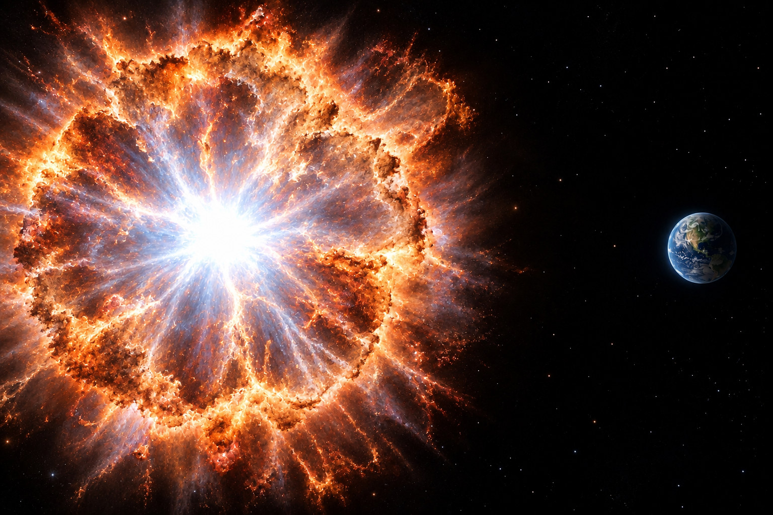
Hypothetical scenario. AI-generated illustration, not to scale.
It is night. We cannot see the sun.
A sensor measuring radiation reports readings consistent with a supernova, but the sensor is noisy and can have elevated readings even in the absence of a supernova.
What should we conclude?
The setup is xkcd 1132.
The same readings, two questions: how reliable are my measurements (estimates), and how probable is each universe given what I saw.
- The prior $p_\Theta(\theta)$.
- The data $\bx$ and the likelihood $p_{\bX|\Theta}(\bx|\theta)$.
- The posterior \[\cpo{p_{\Theta|\bX}(\theta|\bx)}=\frac{\cpr{p_\Theta(\theta)}\,\clk{p_{\bX|\Theta}(\bx|\theta)}}{p_{\bX}(\bx)},\qquad\text{written } \cpo{p(\theta|\bx)}=\frac{\cpr{p(\theta)}\clk{p(\bx|\theta)}}{p(\bx)}\] once the argument makes the distribution clear.
- Recognize the distribution (today's route).
- Integrate numerically.
- Approximate: Markov chain Monte Carlo and variational inference, later in the course.
A road has light traffic on a day with probability $\theta$. Over 10 days, 6 had light traffic. Three steps lead to the posterior.
The mode is 0.6, the MLE; the mean is $7/12=0.583$; the standard deviation is 0.137.
Let $X_i=1$ denote a head and $X_i=0$ a tail, with $X_i\mid\Theta=\theta\sim\ber(\theta)$. The prior on $\Theta$ is uniform.
Predict: sketch the posterior after a single head, before computing it.
- (a) Observe $X_1=1$. Find $p(\theta\mid X_1=1)$.
- (b) Observe $\bx=(1,1,0)$. Find the posterior and $\pr(\Theta>1/2\mid\bX=\bx)$.
- (a) Observe $X_1=1$. Find $p(\theta\mid X_1=1)$.
- (b) Observe $\bx=(1,1,0)$. Find the posterior and $\pr(\Theta>1/2\mid\bX=\bx)$.
A head multiplies the curve by $\theta$ and tilts it right; a tail by $1-\theta$ and tilts it left.
Let $n=h+t$, where $h$ is the number of heads and $t$ the number of tails.
| Proportional form | Named distribution | |
|---|---|---|
| Prior | $\cpr{p(\theta)\propto\theta^{\alpha-1}(1-\theta)^{\beta-1}}$ | $\cpr{\Theta\sim\bet(\alpha,\beta)}$ |
| Likelihood for data $(h,t)$ | $\clk{p(\bx\mid\theta)\propto\theta^h(1-\theta)^t}$ | $\clk{X\mid\Theta\sim\bin(n,\theta)}$ |
| Posterior | $\cpo{p(\theta\mid\bx)\propto\theta^{\cpr{\alpha}+\clk{h}-1}(1-\theta)^{\cpr{\beta}+\clk{t}-1}}$ | $\cpo{\Theta\mid\bx\sim\bet(\cpr{\alpha}+\clk{h},\cpr{\beta}+\clk{t})}$ |
The observed counts add to the two Beta parameters.
A fraction $\theta$ of viewers like a video; the prior is uniform. Call the video high quality if $\theta>0.8$.
Before the data: what is the prior probability that the video is high quality?
After observing $\bx$, use
\[\pr(\Theta>0.8\mid\bx)=\int_{0.8}^1\cpo{p(\theta|\bx)}\,d\theta.\]Predict: which result makes you most confident that the video is high quality?
- (a) 1 like, 0 dislikes: $100\%$ liked it.
- (b) 9 likes, 1 dislike: $90\%$ liked it.
- (c) 85 likes, 15 dislikes: $85\%$ liked it.
Under the uniform prior, $\pr(\Theta>0.8)=1-0.8=0.20$.
| Data $(h,t)$ | Observed rate $h/n$ | Posterior | $\pr(\Theta>0.8\mid\bx)$ |
|---|---|---|---|
| $(1,0)$ | $1.00$ | $\cpo{\bet(2,1)}$ | $0.36$ |
| $(9,1)$ | $0.90$ | $\cpo{\bet(10,2)}$ | $0.68$ |
| $(85,15)$ | $0.85$ | $\cpo{\bet(86,16)}$ | $0.88$ |
Predict: after 100 viewers (80 likes, 20 dislikes), how far apart are the two means? After 1000?
| viewers | flat prior | skeptic $\bet(2,8)$ | gap |
|---|---|---|---|
| 5 | 0.71 | 0.40 | 0.31 |
| 20 (16 likes) | 0.77 | 0.60 | 0.17 |
| 100 (80 likes) | 0.79 | 0.75 | 0.05 |
| 1000 (800 likes) | 0.80 | 0.79 | 0.01 |
Let $\bx$ be the data already observed and $\bx'$ the new data. Assume $\bX'\independent\bX\mid\Theta$, so $\clk{p(\bx'\mid\theta,\bx)}=\clk{p(\bx'\mid\theta)}$.
Road: $\bx$ is the first 10 days (6 light), $\bx'$ the next 40 days (23 light).
For $\alpha,\beta\geq1$, interpret the prior relative to the uniform $\bet(1,1)$ prior:
\[\underbrace{\alpha-1}_{\text{prior successes}},\qquad\underbrace{\beta-1}_{\text{prior failures}}.\]Total prior pseudocount: $\alpha+\beta-2$.
A parameter below $1$ has no pseudocount interpretation and can place substantial mass near a boundary.
Question: which curve fits each setting?
- (a) Little is known about traffic.
- (b) An allele causes a disease.
For more on choosing priors, read about Jeffreys priors.
Let $Y_i$ be the number of events in observation window $i$.
\[\clk{Y_i\mid\Lambda=\lambda\sim\poi(\lambda),\qquad p(y_i\mid\lambda)=e^{-\lambda}\frac{\lambda^{y_i}}{y_i!}}.\]Here, $\lambda$ is the expected count in one window:
\[\E[Y_i\mid\lambda]=\lambda,\qquad\var(Y_i\mid\lambda)=\lambda.\]For $n$ independent windows, let $S=\sum_{i=1}^n y_i$. The Gamma distribution uses the shape–rate parameterization.
| Proportional form | Named distribution | |
|---|---|---|
| Prior | $\cpr{p(\lambda)\propto\lambda^{\alpha-1}e^{-\beta\lambda}}$ | $\cpr{\Lambda\sim\gam(\alpha,\beta)}$ |
| Likelihood for data $y_1^n$ | $\clk{p(y_1^n\mid\lambda)\propto\lambda^S e^{-n\lambda}}$ | $\clk{Y_i\mid\Lambda\sim\poi(\lambda)}$ |
| Posterior | $\cpo{p(\lambda\mid y_1^n)\propto\lambda^{\alpha+S-1}e^{-(\beta+n)\lambda}}$ | $\cpo{\Lambda\mid y_1^n\sim\gam(\alpha+S,\beta+n)}$ |
$\clk{S}$ adds to the Gamma shape, and $\clk{n}$ adds to the Gamma rate.
| Data | $\clk{n=10}$, $\clk{S=20}$ |
| Reference prior | $\cpr{p(\lambda)\propto1}$, $\lambda>0$ |
| Posterior | $\cpo{\Lambda\mid y_1^{10}\sim\gam(21,10)}$ |
| Posterior mean | $\cpo{\E[\Lambda\mid y_1^{10}]=2.1}$ |
“Flat” depends on the parameterization.
Sometimes we need a single number to summarize the posterior distribution.
The choice depends on the loss function.
| Posterior loss | Best estimate |
|---|---|
| $\E[(\Theta-\hat\theta)^2\mid\bx]$ | posterior mean $\E[\Theta|\bx]$ |
| $\E[|\Theta-\hat\theta|\mid\bx]$ | posterior median |
| discrete $0$–$1$ loss | posterior mode |
For continuous $\Theta$, MAP maximizes the posterior density:
\[\hat\theta_{\mathrm{MAP}}=\arg\max_\theta \cpo{p(\theta\mid\bx)},\qquad\hat\theta_{\mathrm{mean}}=\E[\Theta\mid\bx].\]mode 0.020 < median 0.026 < mean 0.029
With $\bar\theta=\E[\Theta|\bx]$,
\[\E[(\hat\theta-\Theta)^2|\bx]=\var(\Theta\mid\bx)+(\hat\theta-\bar\theta)^2.\]The cross term is zero because $\E[\Theta-\bar\theta\mid\bx]=0$.
The loss is minimized at $\hat\theta=\bar\theta$.
Let $\cpo{\Theta\mid\bx\sim\bet(a,b)}$, where $a=\cpr{\alpha}+\clk{h}$ and $b=\cpr{\beta}+\clk{t}$.
The median approximation and the mode formula assume $a,b>1$.
The posterior mean is a weighted average of the MLE and the prior mean:
\[\cpo{\frac{h+\alpha}{n+\alpha+\beta}}=\clk{\frac{n}{n+\alpha+\beta}\cdot\frac{h}{n}}+\cpr{\frac{\alpha+\beta}{n+\alpha+\beta}\cdot\frac{\alpha}{\alpha+\beta}}.\]Given: $n=3$, $h=2$, $t=1$, and $\cpr{\Theta\sim\bet(2,2)}$.
- (a) The posterior?
- (b) Posterior mean, posterior mode, the MLE, the prior mean?
- (c) Check the weighted average.
(a) $\cpo{p(\theta\mid\bx)\propto\theta^3(1-\theta)^2}$, $\cpo{\Theta\mid\bx\sim\bet(4,3)}$.
(b) mean $=4/7$, MAP $=3/5$, MLE $=2/3$, prior mean $=1/2$.
prior .500 mean .571 MAP .600 MLE .667
A fire department has recorded $20$ incidents in $10$ days. With the flat prior, $\cpo{\Lambda\mid y_1^{10}\sim\gam(21,10)}$.
Question: what is $\pr(Y_{11}>5\mid y_1^{10})$, the probability of more than $5$ incidents tomorrow?
The posterior describes $\Lambda$, not tomorrow's count.
For a given rate,
\[\clk{\pr(Y_{11}>5\mid\Lambda=\lambda)=1-\sum_{k=0}^{5}e^{-\lambda}\frac{\lambda^k}{k!}},\]which is $0.004$ at $\lambda=1.5$ and $0.084$ at $\lambda=3$, both plausible rates.
So how do we find the probability of more than $5$ incidents tomorrow, given the data?
Plug in the posterior mean, $\cpo{\E[\Lambda\mid y_1^{10}]=21/10=2.1}$:
\[\cml{Y_{11}\sim\poi(2.1)},\qquad\cml{\pr(Y_{11}>5)=0.020}.\]The posterior still spreads over rates from about $1.3$ to $3.1$ ($95\%$ of its mass). At $\lambda=3$ the same probability is $0.084$, four times larger.
Two distributions are already available:
\[\underbrace{\cpo{p(\lambda\mid y_1^n)}}_{\text{posterior}}\qquad\underbrace{\clk{p(y_{n+1}\mid\lambda)}}_{\text{sampling model}}.\]Average the sampling model over the posterior:
\[\begin{aligned}\cpd{p(y_{n+1}\mid y_1^n)}&=\int p(y_{n+1},\lambda\mid y_1^n)\,d\lambda\\&=\int p(y_{n+1}\mid\lambda,y_1^n)\,\cpo{p(\lambda\mid y_1^n)}\,d\lambda\\&=\int \clk{p(y_{n+1}\mid\lambda)}\,\cpo{p(\lambda\mid y_1^n)}\,d\lambda.\end{aligned}\]Once $\Lambda$ is known, the past does not change the distribution of the next observation.
The last step uses $Y_{n+1}\independent Y_1^n\mid\Lambda$.
Average the Poisson over the posterior $\cpo{\gam(21,10)}$:
\[\cpd{p(y\mid y_1^{10})}=\int\clk{\poi(y;\lambda)}\,\cpo{\gam(\lambda;21,10)}\,d\lambda.\]For the fire department,
\[\cpd{\pr(Y_{11}>5\mid y_1^{10})}=\textstyle\sum_{y>5}\cpd{p(y\mid y_1^{10})}=\cpd{0.026},\]against $\cml{0.020}$ from the plug-in.
Go back to the department's first day: two incidents. With the flat prior, $\cpo{\Lambda\mid y_1\sim\gam(3,1)}$, with posterior mean $3$.
Predict: How does $p(y_2\mid y_1)$ compare to $p(y_2\mid\lambda=3)$?
The plug-in assumes the single rate $\lambda=3$. The posterior predictive includes every plausible rate: each band of rates contributes Poisson counts with its own $\lambda$, weighted by its posterior probability. Variance of tomorrow's count: $\cpd{6}$ for the posterior predictive, $\cml{3}$ for the plug-in.
| plug-in | predictive | |||
|---|---|---|---|---|
| data | variance | $\pr(Y>5)$ | variance | $\pr(Y>5)$ |
| one day, $2$ incidents | $3$ | $0.084$ | $6$ | $0.145$ |
| ten days, $20$ incidents | $2.1$ | $0.020$ | $2.31$ | $0.026$ |
The plug-in is as confident after one day as after ten. The predictive is wide when the data are few and approaches the plug-in as they accumulate.
For counts $\clk{Y_i\mid\Lambda\sim\poi(\Lambda)}$ and posterior $\cpo{\Lambda\mid y_1^n\sim\gam(\alpha+n\bar y,\,\beta+n)}$, the expected count tomorrow follows from iterated expectations:
\[\begin{aligned} \cpd{\E[Y_{n+1}\mid y_1^n]} &= \cpo{\E_{\Lambda\mid y_1^n}}\!\left[ \E(Y_{n+1}\mid\Lambda, y_1^n) \right] && \text{(law of iterated expectations)} \\[2pt] &= \cpo{\E_{\Lambda\mid y_1^n}}\!\left[ \clk{\E(Y_{n+1}\mid\Lambda)} \right] && \text{($Y_{n+1}\independent Y_1^n\mid\Lambda$)} \\[2pt] &= \cpo{\E_{\Lambda\mid y_1^n}[\Lambda]} && \text{($Y_{n+1}\mid\Lambda\sim\poi(\Lambda)\implies\E[Y_{n+1}\mid\Lambda]=\Lambda$)} \\[2pt] &= \cpo{\frac{\alpha+n\bar y}{\beta+n}} && \text{(mean of $\gam(\alpha+n\bar y, \beta+n)$)}. \end{aligned}\]For the one day with two incidents, $\cpo{\gam(3,1)}$ gives $\cpd{\E[Y_2\mid y_1]=3}$.
With $m=\E[\Lambda\mid y_1^n]$, condition on $\Lambda$ as for the mean:
\[\begin{aligned} \cpd{\var(Y_{n+1}\mid y_1^n)} &= \E_{\Lambda\mid y_1^n}\!\left[\E\big((Y_{n+1}-m)^2\mid\Lambda\big)\right] && \text{($Y_{n+1}\independent Y_1^n\mid\Lambda$)} \\[2pt] &= \E_{\Lambda\mid y_1^n}\!\left[\Lambda+(\Lambda-m)^2\right] && \text{($\var(Y_{n+1}\mid\Lambda)=\Lambda$)} \\[2pt] &= \cml{\E[\Lambda\mid y_1^n]}+\cpo{\var(\Lambda\mid y_1^n)}. \end{aligned}\]Next: Gaussian prior and likelihood, with frequentist and Bayesian estimators side by side.